Best answer by MichelleC
View original
How to filter responses by which questions the participant was shown?
I am running a rather complex user study on Qualtrics. I currently have six surveys, and participants are randomly routed to one of the six by clicking the master survey link. This randomly sends them to one of the surveys. Each one has around 100 questions, of which 5 are randomly selected. The issue is with data collection. Exporting the responses shows ALL of the questions (over 600), and I then have to sort through manually to see which ones the participant answered. How can I filter responses and only view which questions the participant saw and answered?

Userlevel 7
 +23
+23
Set up an embedded data with the condition "if this question /or rather any of its options/ is displayed" separately for each of the 5 questions. For example 1 if question 1 is displayed, etc.
Userlevel 7
+23
@mreichar Oh, I am sorry, I somehow misread your message and understood that you want to just see which questions the person answered (like, questions 1, 6, 39, 55, 98). But it will not work as filtering option. Sorry for misleading...

Userlevel 5
 +10
+10
@mreichar, I don't know how to set up a customized export from Qualtrics that will do this, but i know that you can create some custom formatting in Excel.
1. With your exported data file open in Excel, choose the Conditional Formatting menu option.
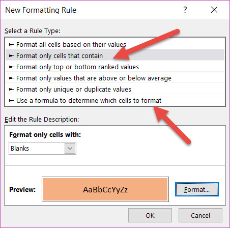
2. Select New Rule
3. Under Select Rule Type, select the Format Only Cells That Contain option
4. Under the Edit Rule Description, change Format Cells with drop down to be Blanks.
5. Click the button to the right of that which says Format. Choose how you want blank cells to be formatted. I chose a Fill color.
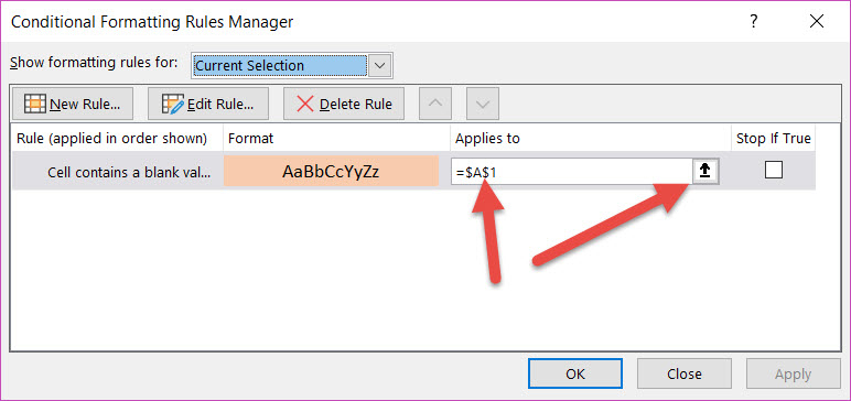
6.When you're done, click Okay and then go back to apply select the range. Go to your Conditional Formatting again and select Manage Rules. You can either type in the cell range or click the small up arrow which will minimize the menu, allowing you to select the entire worksheet with the cursor. Click the down arrow in the minimized menu for it to accept your cell range and then click Okay. It should apply your formatting.
Here's a quick screen shot of the menu:
!
and the Apply To menu:
!
This doesn't automate it perfectly but it should make things hopefully a _little_ easier.
1. With your exported data file open in Excel, choose the Conditional Formatting menu option.
2. Select New Rule
3. Under Select Rule Type, select the Format Only Cells That Contain option
4. Under the Edit Rule Description, change Format Cells with drop down to be Blanks.
5. Click the button to the right of that which says Format. Choose how you want blank cells to be formatted. I chose a Fill color.
6.When you're done, click Okay and then go back to apply select the range. Go to your Conditional Formatting again and select Manage Rules. You can either type in the cell range or click the small up arrow which will minimize the menu, allowing you to select the entire worksheet with the cursor. Click the down arrow in the minimized menu for it to accept your cell range and then click Okay. It should apply your formatting.
Here's a quick screen shot of the menu:
!
and the Apply To menu:
!
This doesn't automate it perfectly but it should make things hopefully a _little_ easier.
Leave a Reply
Enter your username or e-mail address. We'll send you an e-mail with instructions to reset your password.