
User-friendly Guide to Linear Regression
What's on this page
What is Regression?
Regression estimates a mathematical formula that relates one or more input variables to one output variable.
For example, let’s say you run a lemonade stand and you’re interested in what drives revenue. Your data includes each day’s “Revenue,” high “Temperature,” “Number of children who walked by,” “Number of adults who walked by,” what “Signage” you used that day, and a nearby “Competitor’s revenue.”
| Revenue | Temperature (Celsius) | Minutes of Breaktime | Number of children who walked by | Number of adults who walked by | Signage | Competitor’s revenue |
|---|---|---|---|---|---|---|
| $44 | 28.2 | 30 | 43 | 380 | Hand-painted | $20 |
| $23 | 21.4 | 42 | 28 | 207 | LED | $30 |
| $43 | 32.9 | 14 | 43 | 364 | Hand-painted | $34 |
| $30 | 24.0 | 24 | 18 | 103 | LED | $15 |
| etc. | etc. | etc. | etc. | etc. | etc. | etc. |
You think that “Temperature” (an input or explanatory variable) might impact “Revenue” (an output or response variable). When you use regression to analyze this relationship, it might yield this formula:
Revenue = 2.71 * Temperature – 35
This formula is useful for two reasons.
First, it allows you to understand a relationship: hotter days lead to more “Revenue.” In particular, the 2.71 before “Temperature” (called the coefficient) means that for every degree “Temperature” goes up, on average there will be $2.71 more “Revenue.” This insight might lead you to decide not to sell lemonade on cold days.
Second, and relatedly, it can also help you make specific predictions. If the “Temperature” is 24, you could estimate that since…
Revenue = 2.71 * Temperature – 35
Revenue = 2.71 * 24 – 35
Revenue = 30
…you’ll have around $30 in “Revenue.” That might be useful information for knowing whether you’ll be able to make a payment that day, assuming you’re confident that your model is accurate.
Now we’ll walk through the process of creating this regression equation.
Preparing to Create a Regression Model
1. Think through the theory of your regression
Once you’ve chosen a response variable, “Revenue,” hypothesize how various inputs may be related to it. For example, you might think that higher “Temperature” will lead to higher “Revenue,” you might be unsure about how various signage will affect “Revenue,” and you might believe that “Competitor’s sales” are affected by “Temperature” but don’t have any impact on your lemonade stand.
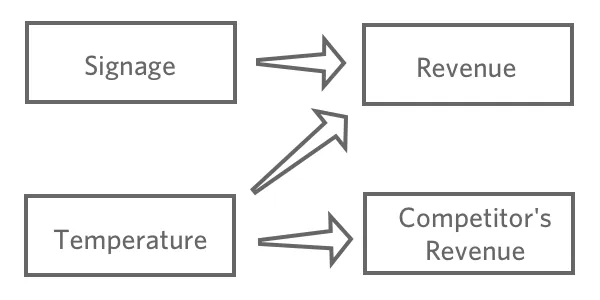
The goal of regression is typically to understand the relationship between several inputs and one output, so in this case you’d probably decide to create a model explaining “Revenue” with “Temperature” and “Signage” (also said as “predicting Revenue from Temperature and Signage“, even if you’re more interested in explanation than actual prediction).
You probably wouldn’t include “Competitor’s sales” in your regression. It’s likely correlated with “Revenue,” but it doesn’t come before it in the causal chain, so including it would confuse your model.
2. “Describe” all variables that could be at all useful for your model
Start by describing the response variable, in this case “Revenue,” and getting a good feel for it. Do the same for your explanatory variables.
Note which have a shape like this…
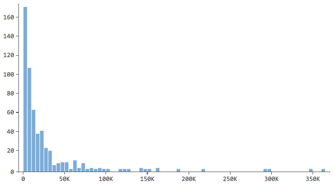

…where most of the data is in the first few bins of the histogram. Those variables will require special attention later.
3. “Relate” all the possible explanatory variables to the response variable
Stats iQ will order the results by the strength of the statistical relationship. Take a look and get a feel for the results, noting which variables are related to “Revenue” and how.
If you already have a good idea of which variables should theoretically drive the output (say, from previous academic papers), you should skip this step. But if your analysis is a bit more exploratory in nature (like a customer survey), this is a useful and important step.
4. Start building the regression
Building a regression model is an iterative process. You’ll cycle through the following three stages as many times as necessary.
The Three Stages of Building a Regression Model
Stage 1: Add or subtract a variable
One by one, start adding in variables that your previous analyses indicated were related to “Revenue” (or add in variables that you have a theoretical reason to add). Going one by one isn’t strictly necessary, but it makes it easier to identify and fix problems as you go along and helps you get a feel for the model.
Let’s say you start by predicting “Revenue” with “Temperature.” You find a strong relationship, you assess the model, and you find it to be satisfactory (more details in a minute).
Revenue = 2.71 * Temperature – 35
You then add in “Number of children who walked by” and now your regression model has two terms, both of which are statistically significant predictors. Like this:
Revenue = 2.5 * Temperature + 0.3 * NumberOfChildrenWhoWalkedBy – 12
Then you add “Number of adults who walked by,” and the model results now show that “Number of adults” is statistically significant in the model, but “Number of children” no longer is. Typically you’d remove “Number of children” from the model. Now we have:
Revenue = 2.6 * Temperature + 0.4 * NumberOfAdultsWhoWalkedBy – 14
This means that “Number of adults” is the better predictor of “Revenue”; that is, if you know how many adults come by, knowing how many children come by doesn’t add any new information – it doesn’t help you predict sales.
Maybe you think back and remember that children don’t really ever buy your lemonade, so it makes sense that that variable doesn’t belong in the model.
Why was it statistically significant in the first model, though? Probably because “Number of children” is correlated with “Number of adults,” and since “Number of adults” wasn’t yet in the model, “Number of children” was acting as a rough proxy for “Number of adults.”
Interpreting regression results takes a good deal of judgment, and just because a variable is statistically significant doesn’t mean it’s actually causal. But by carefully adding and subtracting variables, noting how the model changes, and always thinking about the theory behind your model, you can tease apart interesting relationships in your data.
Stage 2: Assess the model
Every time you add or subtract a variable, you should assess the model’s accuracy by looking at its r-squared (R2), AICR, and its residual plots. Every time you change the model, compare the new r-squared, AICR, and residual plots to the old ones to determine whether the model has improved or not.
R-squared (R2)
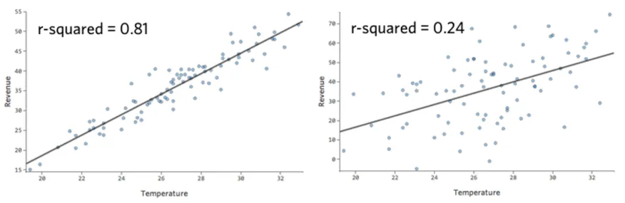
The numeric metric for quantifying the model’s prediction accuracy is known as r-squared, which falls between zero and one. A zero means that the model has no predictive value, and a one means that the model perfectly predicts everything.
For example, the model on the left is more accurate than the one on the right; that is, if you know “Temperature,” you have a pretty good guess as to what “Revenue” will be on the left, but not really on the right.
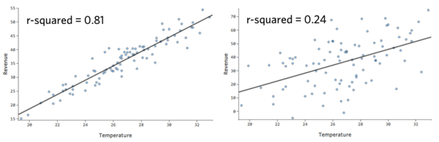
There’s no fixed definition of a “good” r-squared. In some settings it might be interesting to see any effect at all, while in others your model might be useless unless it’s highly accurate.
Any time you add a variable, r-squared will go up, so achieving the highest possible r-squared isn’t the goal; rather, you want to balance the model’s accuracy (r-squared) with its complexity (generally, the number of variables in it).
AICR
AICR is a metric that balances accuracy with complexity – greater accuracy leads to better scores, added complexity (more variables) leads to worse scores. The model with the lower AICR is better.
Note that the AICR metric is only useful for comparing AICRs from models that have the same number of rows of data and the same output variable.
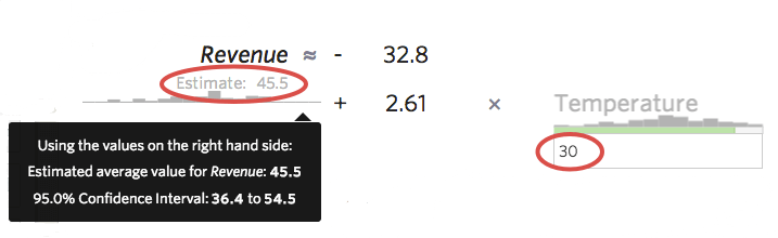
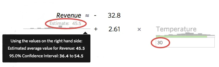
Prediction intervals
Another useful way to get a feel for the accuracy of your model is to stick sample values into your formula and see the prediction interval that Stats iQ computes. For example, if you stick the number 30 into the formula, Stats iQ will tell you that the predicted value is 45.5, but the 95% confidence interval is 36.4 to 54.5, meaning that you could be 95% sure that if tomorrow turned out to be 30 degrees, you’d get between $36.40 and $54.50 in “Revenue.” You could imagine a more accurate model where the prediction interval was a tight band like $44 to $48, or a less accurate one where the interval was wide, like $20 to $72.
This approach is only helpful when your residual plots look healthy (see below), otherwise they’ll be inaccurate.
Residuals
Residuals are the primary diagnostic tool for assessing and improving regression, so there’s a whole separate section on interpreting residuals to improve your model. You’ll learn or refresh your memory about what residuals are, how to use them to assess and improve the model, and how to think about how accurate you need your model to be.
We recommend you read it in full, as it’ll cover everything else you need to produce a great model. But you can always come back to it, of course.
Stage 3: Modify the model accordingly
If your assessment of the model found it to be satisfactory, you’re either done, or you can go back to Stage 1 and enter more variables.
If your assessment finds the model lacking, you’ll use Stats iQ’s alerts and the residual diagnostic section to fix the issues.
As you modify the model, continually note the changing r-squared, AICR, and residual diagnostics, and decide whether the changes you’re making are helping or hurting your model.
FAQs
How do I create a new Stats iQ variable?
How do I create a new Stats iQ variable?
What are the options for analyzing my data in Stats iQ?
What are the options for analyzing my data in Stats iQ?
- Describe: Selecting a variable from the list and then clicking Describe will give you a visualization of the data contained in that variable. Use this when you would like to see how the data for a certain variable is distributed.
- Relate: Selecting two variables and then clicking Relate will run a statistical analysis of the relation between the two variables. Use this when you would like to know how strongly two variables are correlated.
- Pivot Table: Selecting two or more variables and clicking Pivot Table will create a table that displays the values of the variables as rows and columns. The cells can be set to display a variety of different information including column and row percentage, Sum, and Variance. Use this when you would like to compare the overlap between specific values of a set of variables.
- Regression: Selecting two variables and clicking Regression will give the mathematical relationship between the variables. Use this when you would like to predict values for one variable based off of the values of another.
- Cluster: Selecting two to ten demographic variables and clicking Cluster will display groupings of traits most likely to occur together, thus revealing the population segments captured in your data.
I don't know what this statistical term means. Can you tell me?
I don't know what this statistical term means. Can you tell me?
- Statistical tests: ANOVA, T-test, and Chi-squared are all statistical test that Stats iQ performs to test whether or not the relationship between two variables is significant. These tests are used to generate a P-Value.
- P-Value: This value represents the probability that the observed results would be seen if no correlation between the variables exists. A lower P-Value means more correlated data.
- Effect Size: The effect size is a measure of how large the correlation between two variables is. This is measured in different ways depending on the type of the statistical test performed. Examples are Cohen’s d, Pearson’s r, and Cramer’s v. The larger the effect size value, the more correlated the variables are.
How do I filter the data that appears in Stats iQ?
How do I filter the data that appears in Stats iQ?
How do I get my new responses to show up in Stats iQ?
How do I get my new responses to show up in Stats iQ?
How are analysis cards ordered in my Stats iQ Workspace?
How are analysis cards ordered in my Stats iQ Workspace?
What’s Stats iQ? / Where’s Statwing?
What’s Stats iQ? / Where’s Statwing?
What do I do if my data isn't loading properly?
What do I do if my data isn't loading properly?
That's great! Thank you for your feedback!
Thank you for your feedback!