
Interpreting Residual Plots to Improve Your Regression
What's on this page
When you run a regression, Stats iQ automatically calculates and plots residuals to help you understand and improve your regression model. Read below to learn everything you need to know about interpreting residuals (including definitions and examples).
Observations, Predictions, and Residuals
To demonstrate how to interpret residuals, we’ll use a lemonade stand dataset, where each row was a day of “Temperature” and “Revenue.”
| Temperature (Celsius) | Revenue |
|---|---|
| 28.2 | $44 |
| 21.4 | $23 |
| 32.9 | $43 |
| 24.0 | $30 |
| etc. | etc. |
The regression equation describing the relationship between “Temperature” and “Revenue” is:
Revenue = 2.7 * Temperature – 35
Let’s say one day at the lemonade stand it was 30.7 degrees and “Revenue” was $50. That 50 is your observed or actual output, the value that actually happened.
So if we insert 30.7 at our value for “Temperature”…
Revenue = 2.7 * 30.7 – 35
Revenue = 48
…we get $48. That’s the predicted value for that day, also known as the value for “Revenue” the regression equation would have predicted based on the “Temperature.”
Your model isn’t always perfectly right, of course. In this case, the prediction is off by 2; that difference, the 2, is called the residual. The residual is the bit that’s left when you subtract the predicted value from the observed value.
Residual = Observed – Predicted
You can imagine that every row of data now has, in addition, a predicted value and a residual.
| Temperature (Celsius) | Revenue (Observed) | Revenue (Predicted) | Residual (Observed – Predicted) |
|---|---|---|---|
| 28.2 | $44 | $41 | $3 |
| 21.4 | $23 | $23 | $0 |
| 32.9 | $43 | $54 | -$11 |
| 24.0 | $30 | $29 | $1 |
| etc. | etc. | etc. | etc. |
We’re going to use the observed, predicted, and residual values to assess and improve the model.
Understanding Accuracy with Observed vs. Predicted
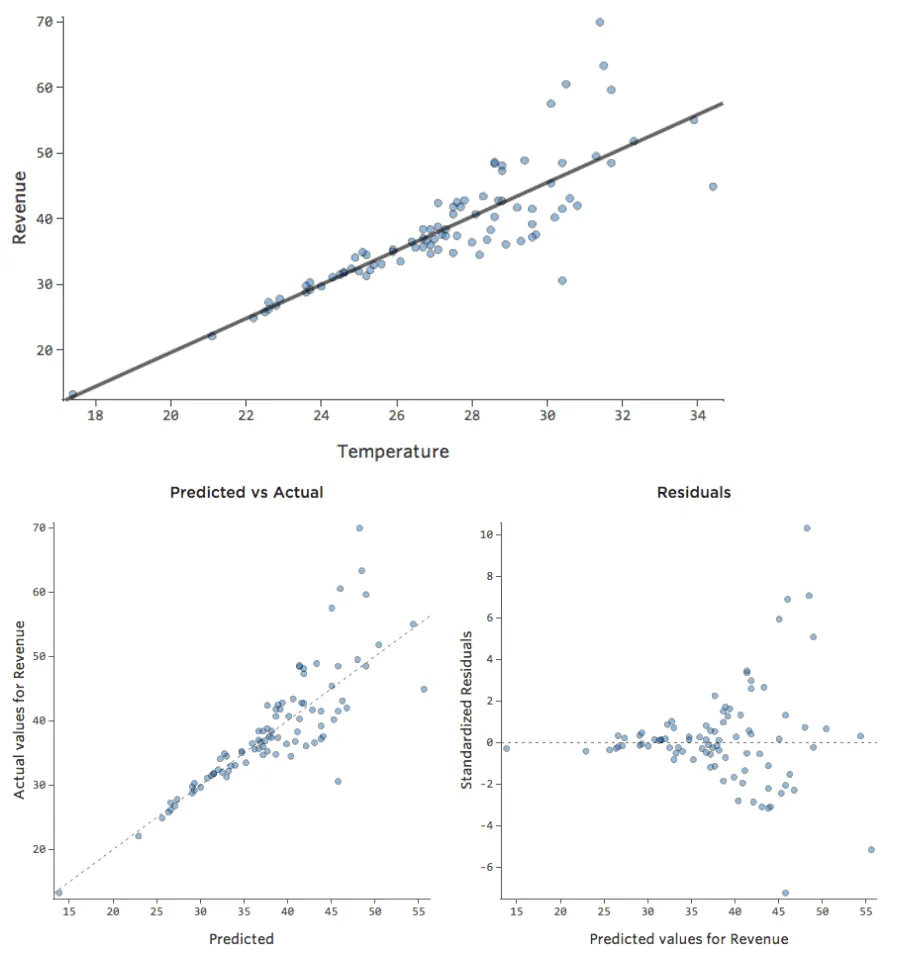
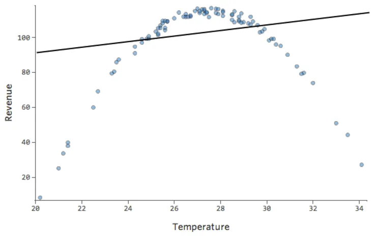
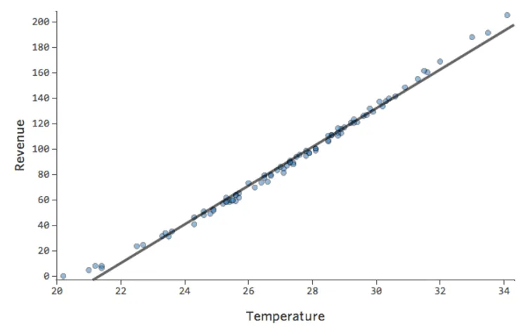
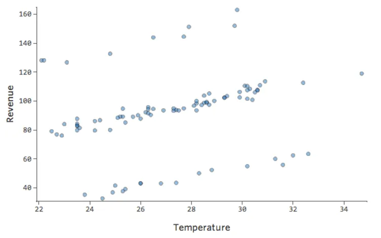
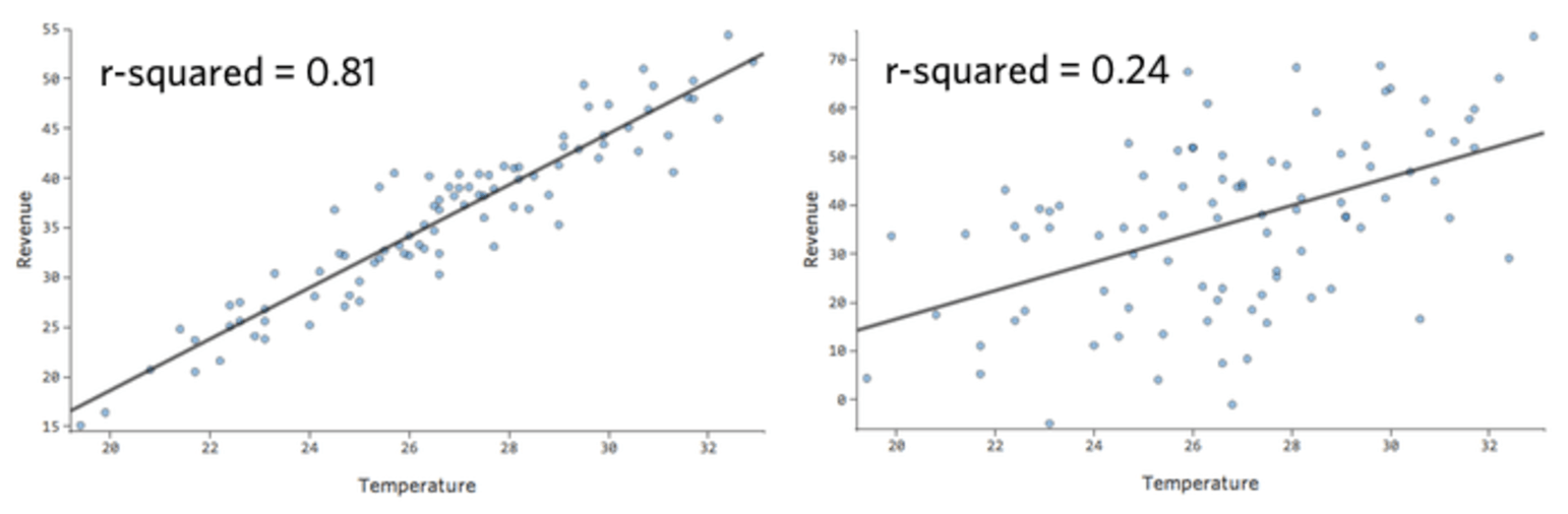
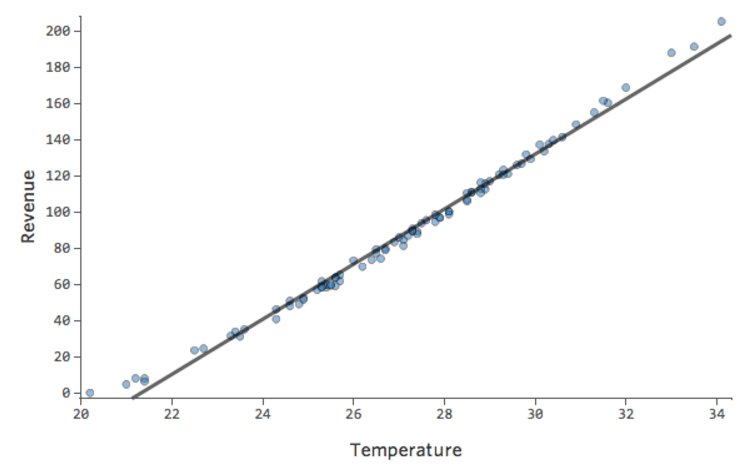
In a simple model like this, with only two variables, you can get a sense of how accurate the model is just by relating “Temperature” to “Revenue.” Here’s the same regression run on two different lemonade stands, one where the model is very accurate, one where the model is not:
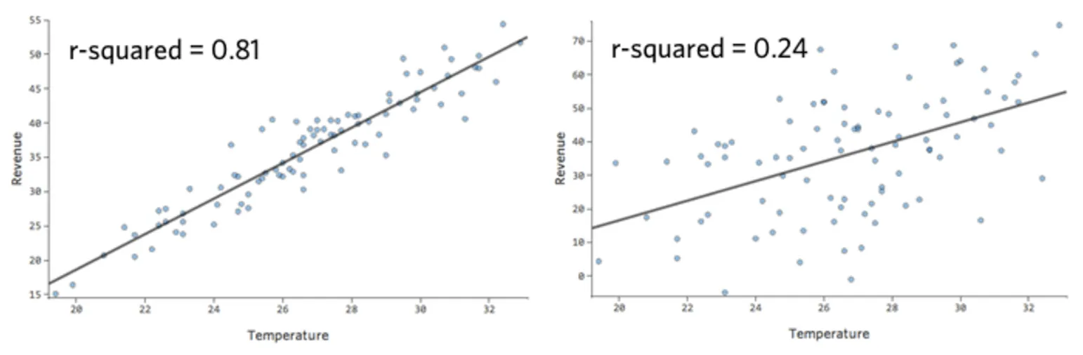
It’s clear that for both lemonade stands, a higher “Temperature” is associated with higher “Revenue.” But at a given “Temperature,” you could forecast the “Revenue” of the left lemonade stand much more accurately than the right lemonade stand, which means the model is much more accurate.
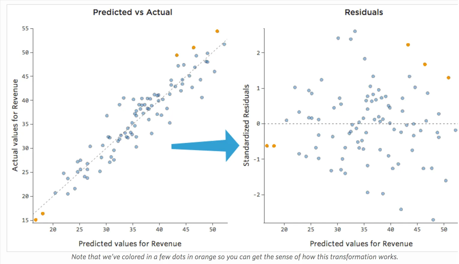
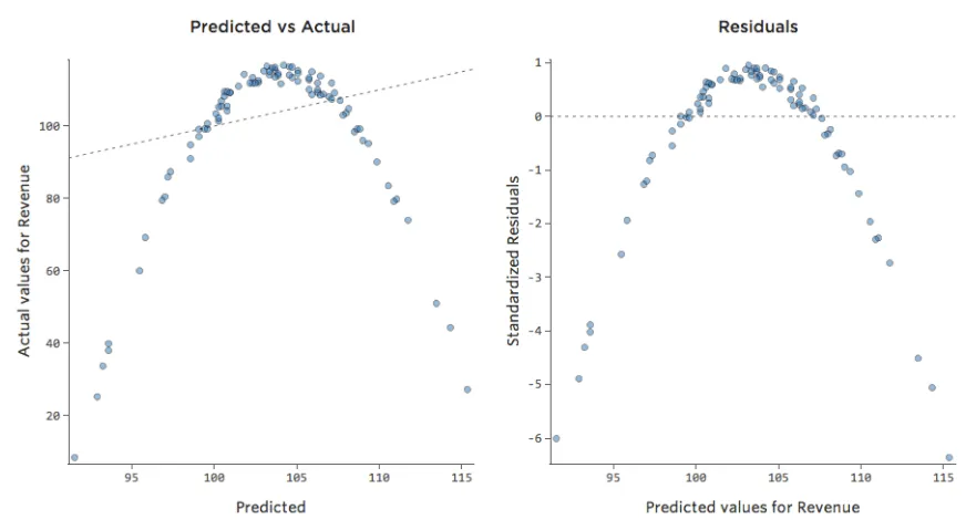
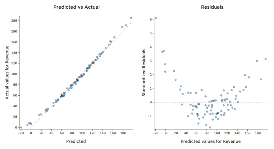
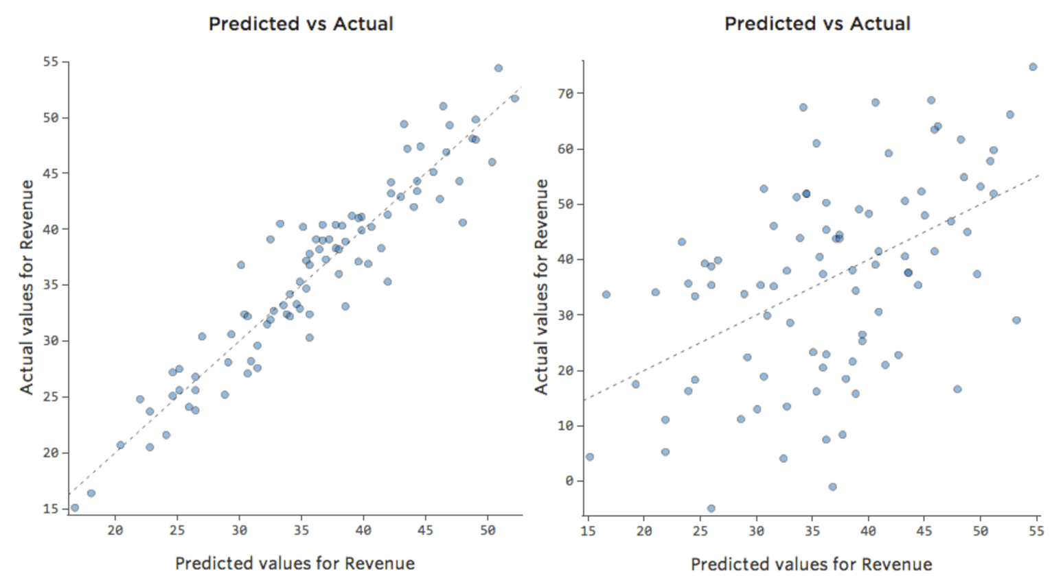
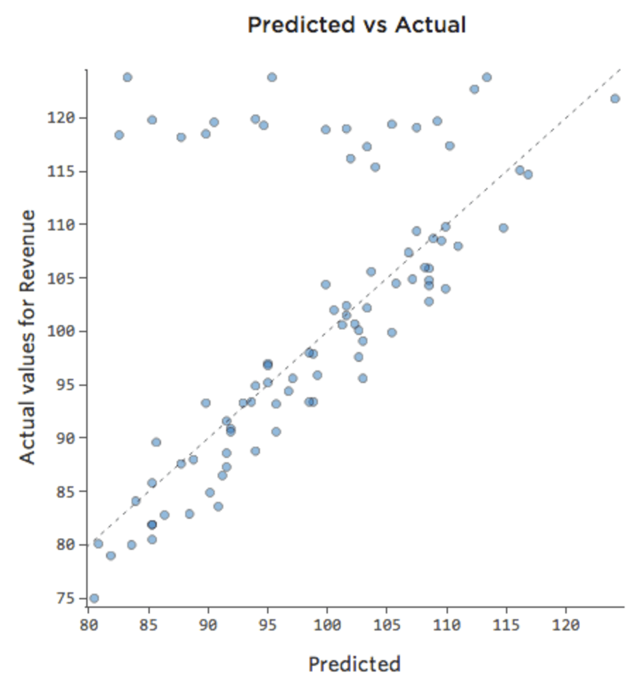
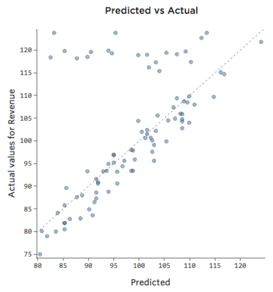
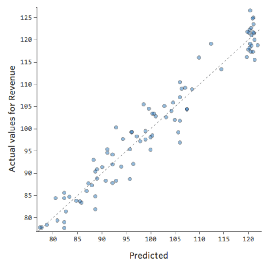
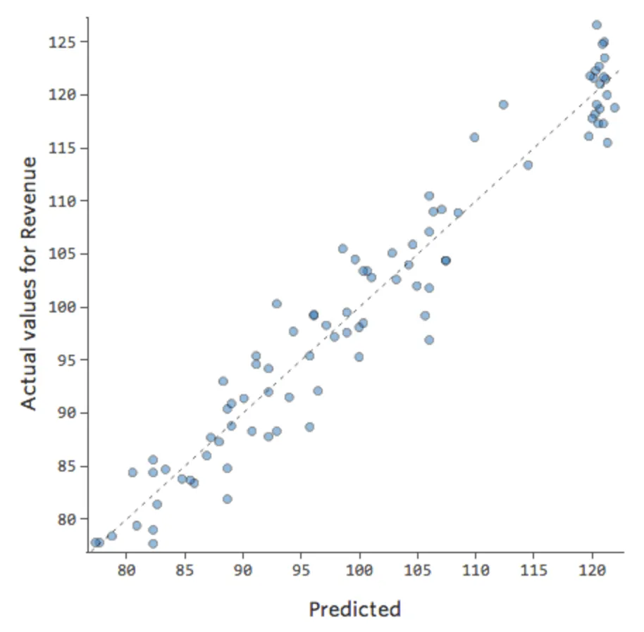
But most models have more than one explanatory variable, and it’s not practical to represent more variables in a chart like that. So instead, let’s plot the predicted values versus the observed values for these same datasets.

Again, the model for the chart on the left is very accurate; there’s a strong correlation between the model’s predictions and its actual results. The model for the chart on the far right is the opposite; the model’s predictions aren’t very good at all.
Note that these charts look just like the “Temperature” vs. “Revenue” charts above them, but the x-axis is predicted “Revenue” instead of “Temperature.” That’s common when your regression equation only has one explanatory variable. More often, though, you’ll have multiple explanatory variables, and these charts will look quite different from a plot of any one explanatory variable vs. “Revenue.”
Examining Predicted vs. Residual (“The Residual Plot”)
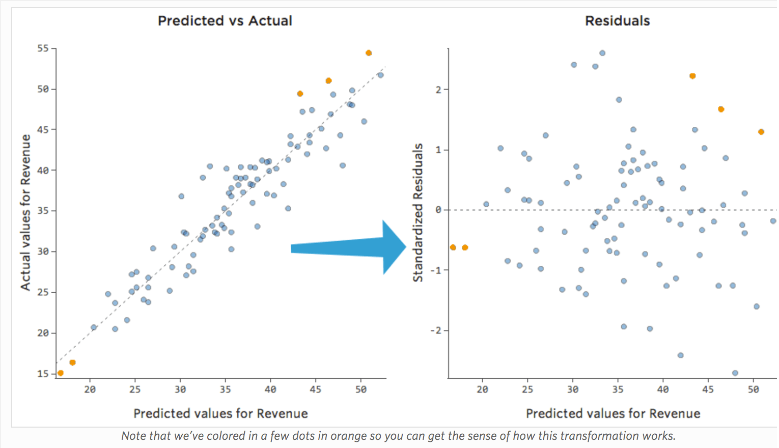
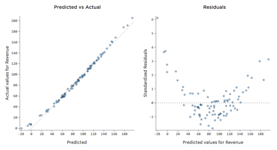
The most useful way to plot the residuals, though, is with your predicted values on the x-axis and your residuals on the y-axis.
(Stats iQ presents residuals as standardized residuals, which means every residual plot you look at with any model is on the same standardized y-axis.)
In the plot on the right, each point is one day, where the prediction made by the model is on the x-axis and the accuracy of the prediction is on the y-axis. The distance from the line at 0 is how bad the prediction was for that value.
Since…
Residual = Observed – Predicted
…positive values for the residual (on the y-axis) mean the prediction was too low, and negative values mean the prediction was too high; 0 means the guess was exactly correct.
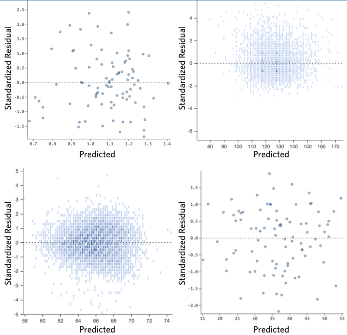
Ideally your plot of the residuals looks like one of these:

That is,
(1) they’re pretty symmetrically distributed, tending to cluster towards the middle of the plot.
(2) they’re clustered around the lower single digits of the y-axis (e.g., 0.5 or 1.5, not 30 or 150).
(3) in general, there aren’t any clear patterns.
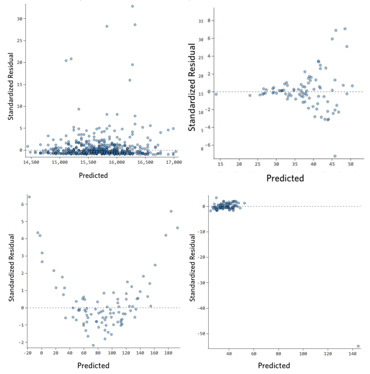
Here’s some residual plots that don’t meet those requirements:
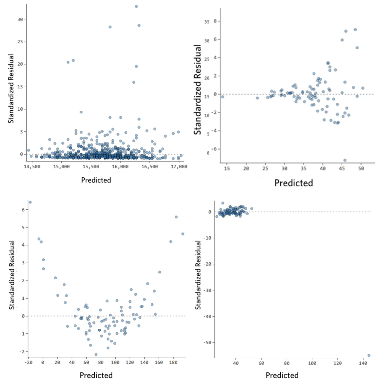
These plots aren’t evenly distributed vertically, or they have an outlier, or they have a clear shape to them.
If you can detect a clear pattern or trend in your residuals, then your model has room for improvement.
In a second we’ll break down why and what to do about it.
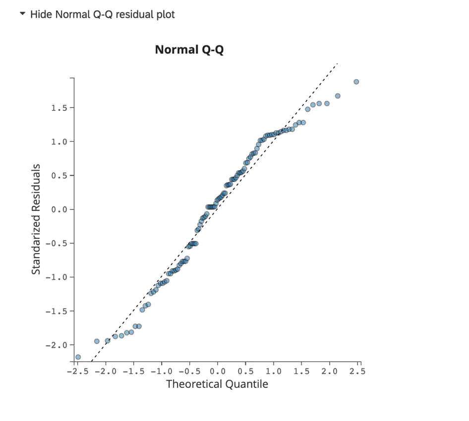
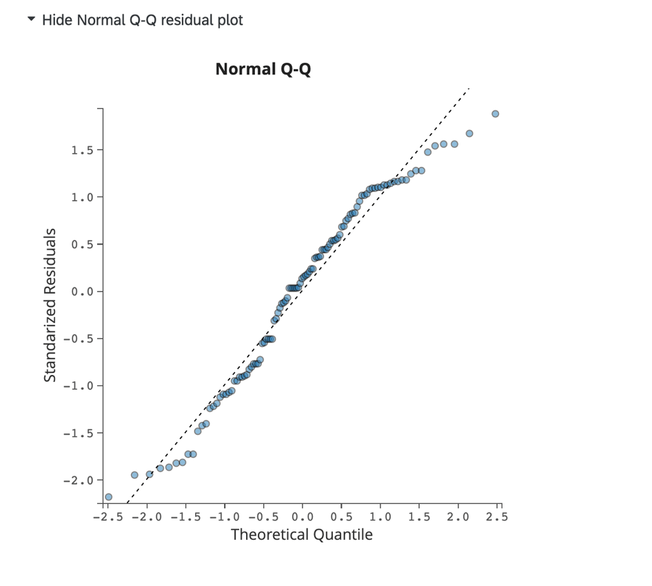
Normal Q-Q Residual Plot:
Click Show Normal Q-Q residual plot to display a Q-Q plot assessing data skew and model fit. This chart displays the standardized residuals on the y-axis and the theoretical quantiles on the x-axis.
How much does it matter if my model isn’t perfect?
How concerned should you be if your model isn’t perfect, if your residuals look a bit unhealthy? It’s up to you.
If you’re publishing your thesis in particle physics, you probably want to make sure your model is as accurate as humanly possible. If you’re trying to run a quick and dirty analysis of your nephew’s lemonade stand, a less-than-perfect model might be good enough to answer whatever questions you have (e.g., whether “Temperature” appears to affect “Revenue”).
Most of the time a decent model is better than none at all. So take your model, try to improve it, and then decide whether the accuracy is good enough to be useful for your purposes.
Example Residual Plots and Their Diagnoses
If you’re not sure what a residual is, take five minutes to read the above, then come back here.
Below is a gallery of unhealthy residual plots. Your residual may look like one specific type from below, or some combination.
If yours looks like one of the below, click that residual to understand what’s happening and learn how to fix it.
(Throughout we’ll use a lemonade stand’s “Revenue” vs. that day’s “Temperature” as an example dataset.)
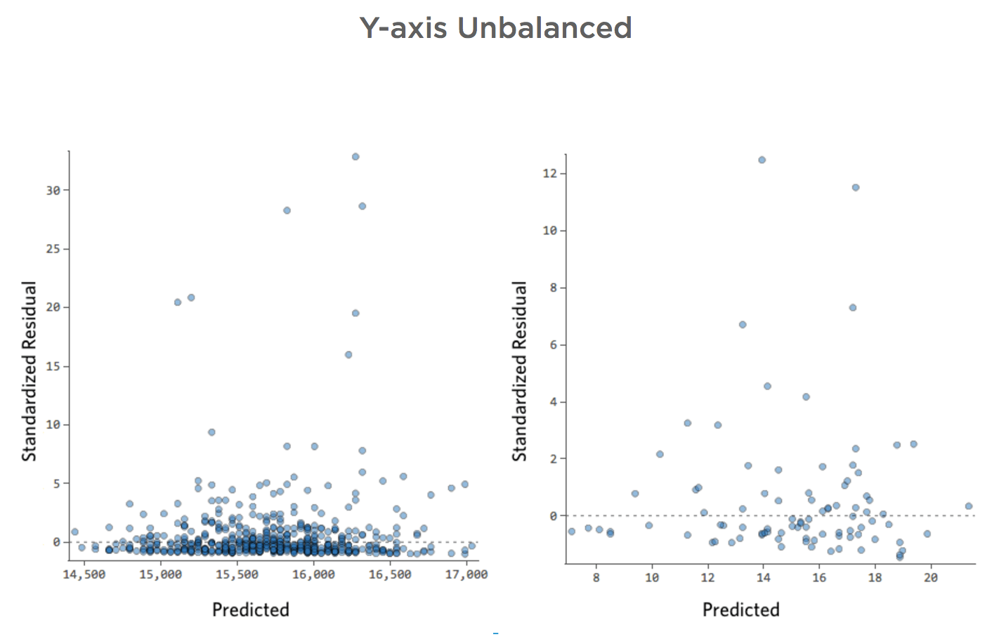
Y-axis Unbalanced

Show details about this plot, and how to fix it.
Show details about this plot, and how to fix it.
Problem
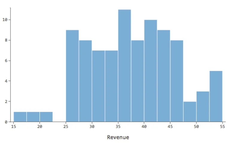
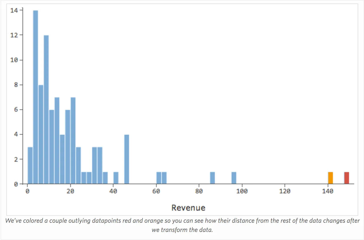
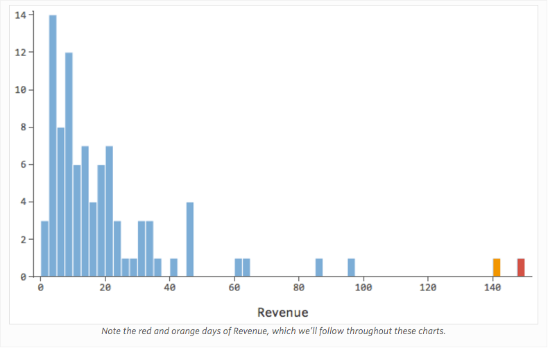
Imagine that for whatever reason, your lemonade stand typically has low revenue, but every once and a while you get very high-revenue days, such that “Revenue” looked like this…

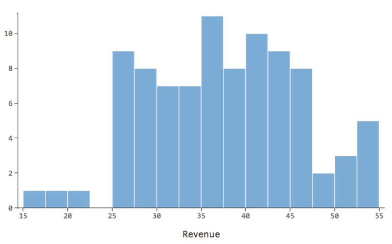
…instead of something more symmetrical and bell-shaped like this:
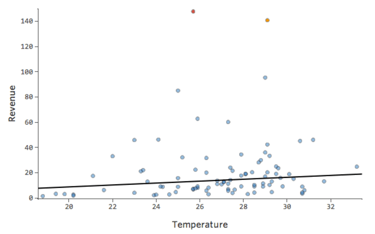
So “Temperature” vs. “Revenue” might look like this, with most of the data bunched at the bottom…

The black line represents the model equation, the model’s prediction of the relationship between “Temperature” and “Revenue.” Look above at each prediction made by the black line for a given “Temperature” (e.g., at “Temperature” 30, “Revenue” is predicted to be about 20). You can see that the majority of dots are below the line (that is, the prediction was too high), but a few dots are very far above the line (that is, the prediction was far too low).
Translating that same data to the diagnostic plots, most of the equation’s predictions are a bit too high, and then some would be way too low.
Implications
This almost always means your model can be made significantly more accurate. Most of the time you’ll find that the model was directionally correct but pretty inaccurate relative to an improved version. It’s not uncommon to fix an issue like this and consequently see the model’s r-squared jump from 0.2 to 0.5 (on a 0 to 1 scale).
How to Fix
- The solution to this is almost always to transform your data, typically your response variable.
- It’s also possible that your model lacks a variable.
Heteroscedasticity
Show details about this plot, and how to fix it.
Show details about this plot, and how to fix it.
Problem
Imagine that for whatever reason, your lemonade stand typically has low revenue, but every once and a while you get very high-revenue days, such that “Revenue” looked like this…
…instead of something more symmetrical and bell-shaped like this:
So “Temperature” vs. “Revenue” might look like this, with most of the data bunched at the bottom…
The black line represents the model equation, the model’s prediction of the relationship between “Temperature” and “Revenue.” Look above at each prediction made by the black line for a given “Temperature” (e.g., at “Temperature” 30, “Revenue” is predicted to be about 20). You can see that the majority of dots are below the line (that is, the prediction was too high), but a few dots are very far above the line (that is, the prediction was far too low).
Translating that same data to the diagnostic plots, most of the equation’s predictions are a bit too high, and then some would be way too low.
Implications
This almost always means your model can be made significantly more accurate. Most of the time you’ll find that the model was directionally correct but pretty inaccurate relative to an improved version. It’s not uncommon to fix an issue like this and consequently see the model’s r-squared jump from 0.2 to 0.5 (on a 0 to 1 scale).
How to Fix
- The solution to this is almost always to transform your data, typically your response variable.
- It’s also possible that your model lacks a variable.
Show details about this plot, and how to fix it.
Show details about this plot, and how to fix it.
Problem
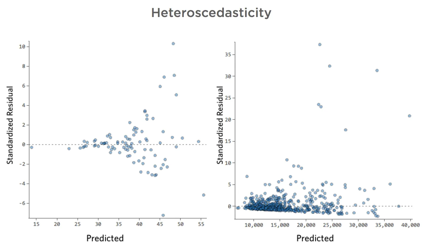
These plots exhibit “heteroscedasticity,” meaning that the residuals get larger as the prediction moves from small to large (or from large to small).
Imagine that on cold days, the amount of revenue is very consistent, but on hotter days, sometimes revenue is very high and sometimes it’s very low.
You’d see plots like these:
Implications
This doesn’t inherently create a problem, but it’s often an indicator that your model can be improved.
The only exception here is that if your sample size is less than 250, and you can’t fix the issue using the below, your p-values may be a bit higher or lower than they should be, so possibly a variable that is right on the border of significance may end up erroneously on the wrong side of that border. Your regression coefficients (the number of units “Revenue” changes when “Temperature” goes up one) will still be accurate, though.
How to Fix
- The most frequently successful solution is to transform a variable.
- Often heteroscedasticity indicates that a variable is missing.
Nonlinear

Show details about this plot, and how to fix it.
Show details about this plot, and how to fix it.
Problem
Imagine that for whatever reason, your lemonade stand typically has low revenue, but every once and a while you get very high-revenue days, such that “Revenue” looked like this…
…instead of something more symmetrical and bell-shaped like this:
So “Temperature” vs. “Revenue” might look like this, with most of the data bunched at the bottom…
The black line represents the model equation, the model’s prediction of the relationship between “Temperature” and “Revenue.” Look above at each prediction made by the black line for a given “Temperature” (e.g., at “Temperature” 30, “Revenue” is predicted to be about 20). You can see that the majority of dots are below the line (that is, the prediction was too high), but a few dots are very far above the line (that is, the prediction was far too low).
Translating that same data to the diagnostic plots, most of the equation’s predictions are a bit too high, and then some would be way too low.
Implications
This almost always means your model can be made significantly more accurate. Most of the time you’ll find that the model was directionally correct but pretty inaccurate relative to an improved version. It’s not uncommon to fix an issue like this and consequently see the model’s r-squared jump from 0.2 to 0.5 (on a 0 to 1 scale).
How to Fix
- The solution to this is almost always to transform your data, typically your response variable.
- It’s also possible that your model lacks a variable.
Show details about this plot, and how to fix it.
Show details about this plot, and how to fix it.
Problem
These plots exhibit “heteroscedasticity,” meaning that the residuals get larger as the prediction moves from small to large (or from large to small).
Imagine that on cold days, the amount of revenue is very consistent, but on hotter days, sometimes revenue is very high and sometimes it’s very low.
You’d see plots like these:
Implications
This doesn’t inherently create a problem, but it’s often an indicator that your model can be improved.
The only exception here is that if your sample size is less than 250, and you can’t fix the issue using the below, your p-values may be a bit higher or lower than they should be, so possibly a variable that is right on the border of significance may end up erroneously on the wrong side of that border. Your regression coefficients (the number of units “Revenue” changes when “Temperature” goes up one) will still be accurate, though.
How to Fix
- The most frequently successful solution is to transform a variable.
- Often heteroscedasticity indicates that a variable is missing.
Show details about this plot, and how to fix it.
Show details about this plot, and how to fix it.
Problem
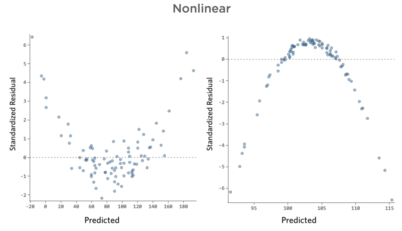
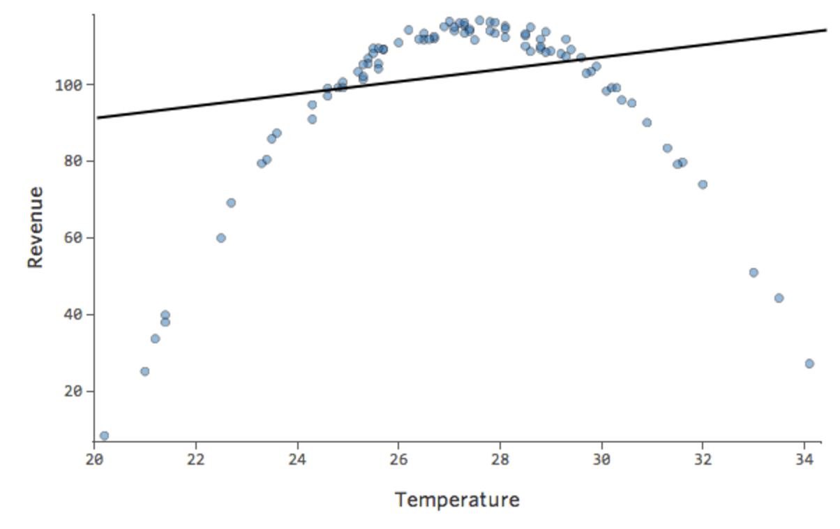
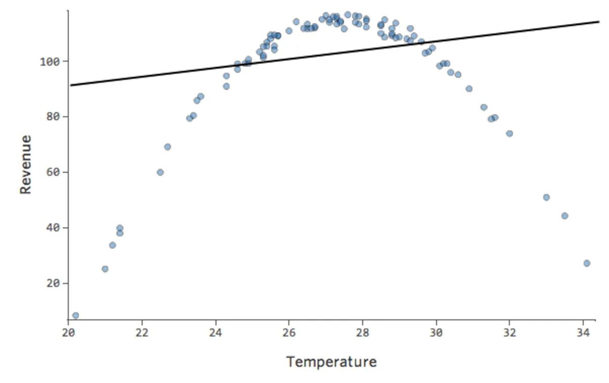
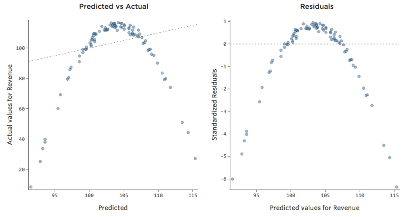
Imagine that it’s hard to sell lemonade on cold days, easy to sell it on warm days, and hard to sell it on very hot days (maybe because no one leaves their house on very hot days).
That plot would look like this:
The model, represented by the line, is terrible. The predictions would be way off, meaning your model doesn’t accurately represent the relationship between “Temperature” and “Revenue.”
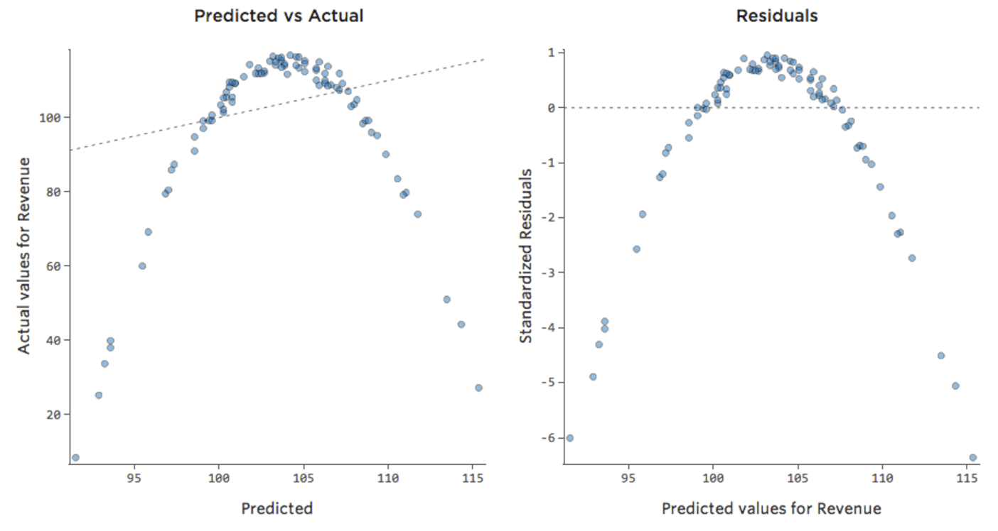
Accordingly, residuals would look like this:
Implications
If your model is way off, as in the example above, your predictions will be pretty worthless (and you’ll notice a very low r-squared, like the 0.027 r-squared for the above).
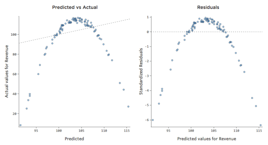
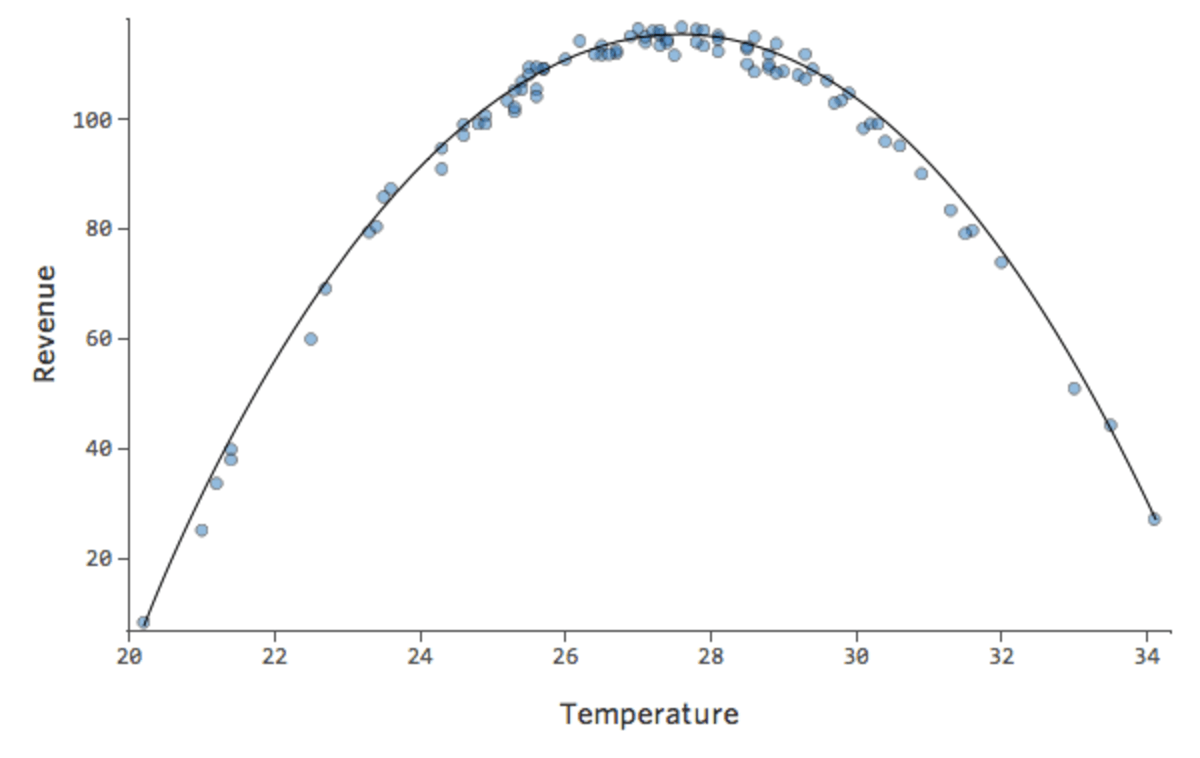
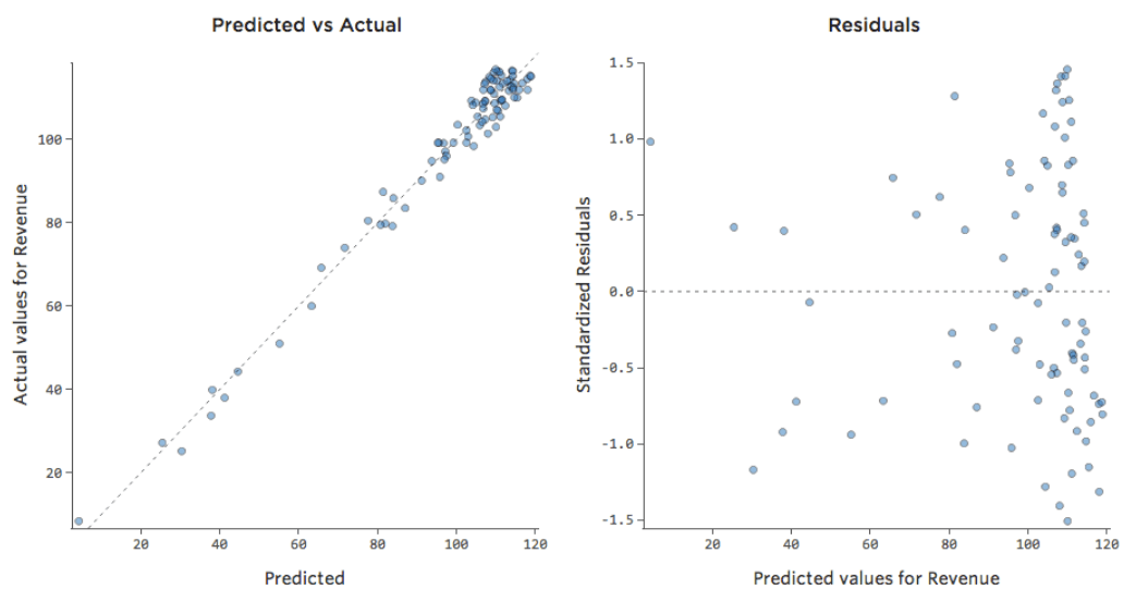
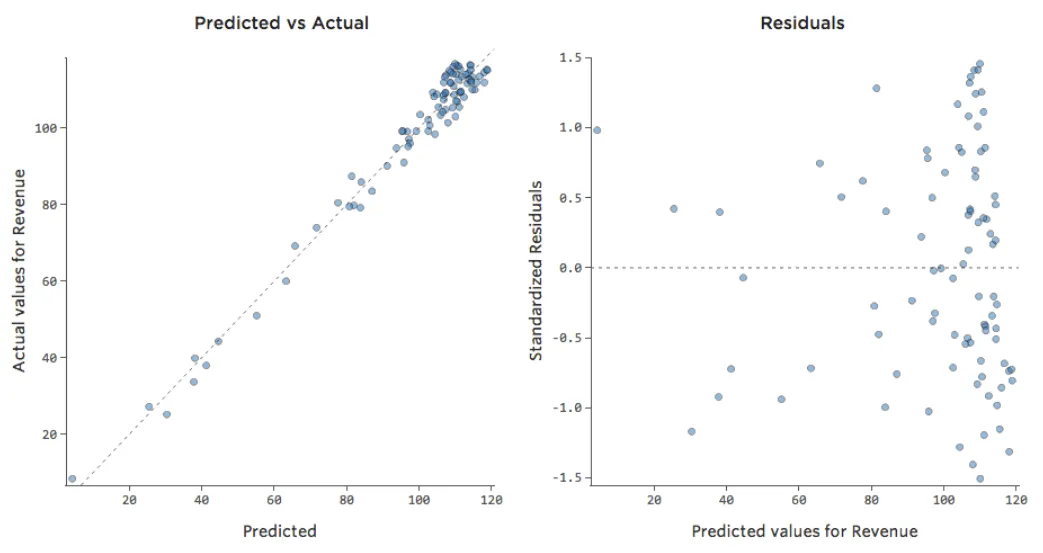
Other times a slightly suboptimal fit will still give you a good general sense of the relationship, even if it’s not perfect, like the below:
That model looks pretty accurate. If you look closely (or if you look at the residuals), you can tell that there’s a bit of a pattern here – that the dots are on a curve that the line doesn’t quite match.
Does that matter? It’s up to you. If you’re getting a quick understanding of the relationship, your straight line is a pretty decent approximation. If you’re going to use this model for prediction and not explanation, the most accurate possible model would probably account for that curve.
How to Fix
- Sometimes patterns like this indicate that a variable needs to be transformed.
- If the pattern is actually as clear as these examples, you probably need to create a nonlinear model (it’s not as hard as that sounds).
- Or, as always, it’s possible that the issue is a missing variable.
Outliers

Show details about this plot, and how to fix it.
Show details about this plot, and how to fix it.
Problem
Imagine that for whatever reason, your lemonade stand typically has low revenue, but every once and a while you get very high-revenue days, such that “Revenue” looked like this…
…instead of something more symmetrical and bell-shaped like this:
So “Temperature” vs. “Revenue” might look like this, with most of the data bunched at the bottom…
The black line represents the model equation, the model’s prediction of the relationship between “Temperature” and “Revenue.” Look above at each prediction made by the black line for a given “Temperature” (e.g., at “Temperature” 30, “Revenue” is predicted to be about 20). You can see that the majority of dots are below the line (that is, the prediction was too high), but a few dots are very far above the line (that is, the prediction was far too low).
Translating that same data to the diagnostic plots, most of the equation’s predictions are a bit too high, and then some would be way too low.
Implications
This almost always means your model can be made significantly more accurate. Most of the time you’ll find that the model was directionally correct but pretty inaccurate relative to an improved version. It’s not uncommon to fix an issue like this and consequently see the model’s r-squared jump from 0.2 to 0.5 (on a 0 to 1 scale).
How to Fix
- The solution to this is almost always to transform your data, typically your response variable.
- It’s also possible that your model lacks a variable.
Show details about this plot, and how to fix it.
Show details about this plot, and how to fix it.
Problem
These plots exhibit “heteroscedasticity,” meaning that the residuals get larger as the prediction moves from small to large (or from large to small).
Imagine that on cold days, the amount of revenue is very consistent, but on hotter days, sometimes revenue is very high and sometimes it’s very low.
You’d see plots like these:
Implications
This doesn’t inherently create a problem, but it’s often an indicator that your model can be improved.
The only exception here is that if your sample size is less than 250, and you can’t fix the issue using the below, your p-values may be a bit higher or lower than they should be, so possibly a variable that is right on the border of significance may end up erroneously on the wrong side of that border. Your regression coefficients (the number of units “Revenue” changes when “Temperature” goes up one) will still be accurate, though.
How to Fix
- The most frequently successful solution is to transform a variable.
- Often heteroscedasticity indicates that a variable is missing.
Show details about this plot, and how to fix it.
Show details about this plot, and how to fix it.
Problem
Imagine that it’s hard to sell lemonade on cold days, easy to sell it on warm days, and hard to sell it on very hot days (maybe because no one leaves their house on very hot days).
That plot would look like this:
The model, represented by the line, is terrible. The predictions would be way off, meaning your model doesn’t accurately represent the relationship between “Temperature” and “Revenue.”
Accordingly, residuals would look like this:
Implications
If your model is way off, as in the example above, your predictions will be pretty worthless (and you’ll notice a very low r-squared, like the 0.027 r-squared for the above).
Other times a slightly suboptimal fit will still give you a good general sense of the relationship, even if it’s not perfect, like the below:
That model looks pretty accurate. If you look closely (or if you look at the residuals), you can tell that there’s a bit of a pattern here – that the dots are on a curve that the line doesn’t quite match.
Does that matter? It’s up to you. If you’re getting a quick understanding of the relationship, your straight line is a pretty decent approximation. If you’re going to use this model for prediction and not explanation, the most accurate possible model would probably account for that curve.
How to Fix
- Sometimes patterns like this indicate that a variable needs to be transformed.
- If the pattern is actually as clear as these examples, you probably need to create a nonlinear model (it’s not as hard as that sounds).
- Or, as always, it’s possible that the issue is a missing variable.
Show details about this plot, and how to fix it.
Show details about this plot, and how to fix it.
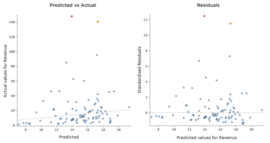
Problem
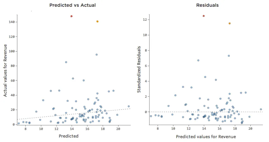
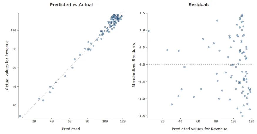
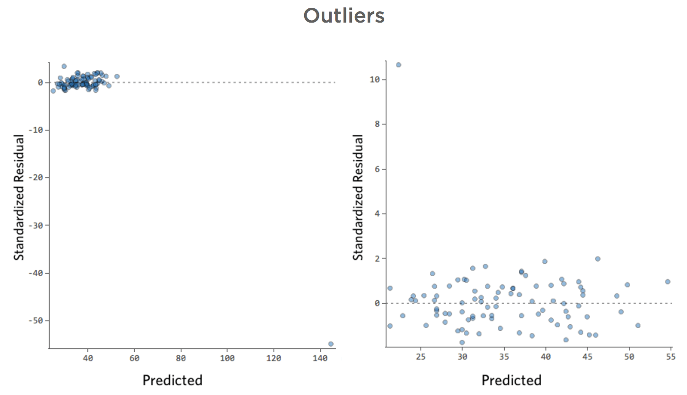
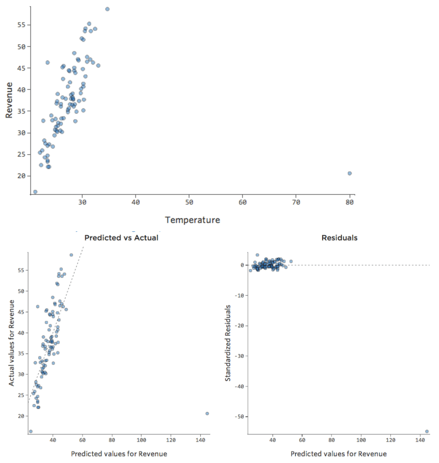
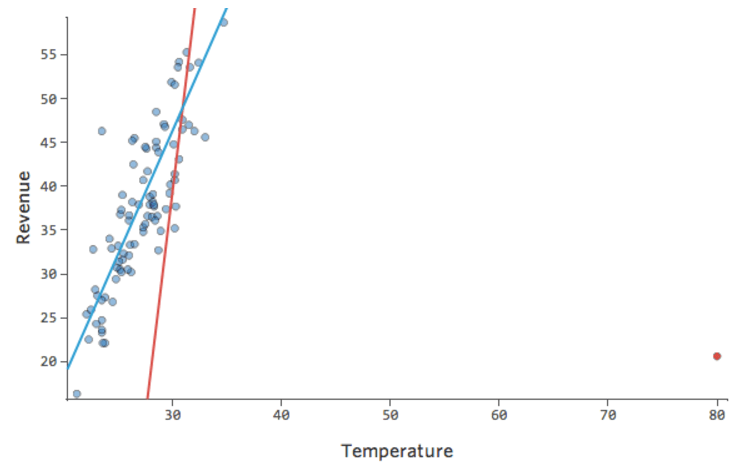
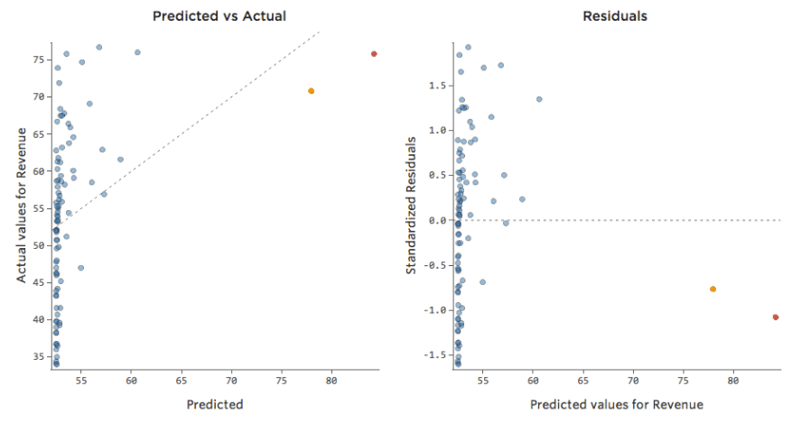
What if one of your datapoints had a “Temperature” of 80 instead of the normal 20s and 30s? Your plots would look like this:
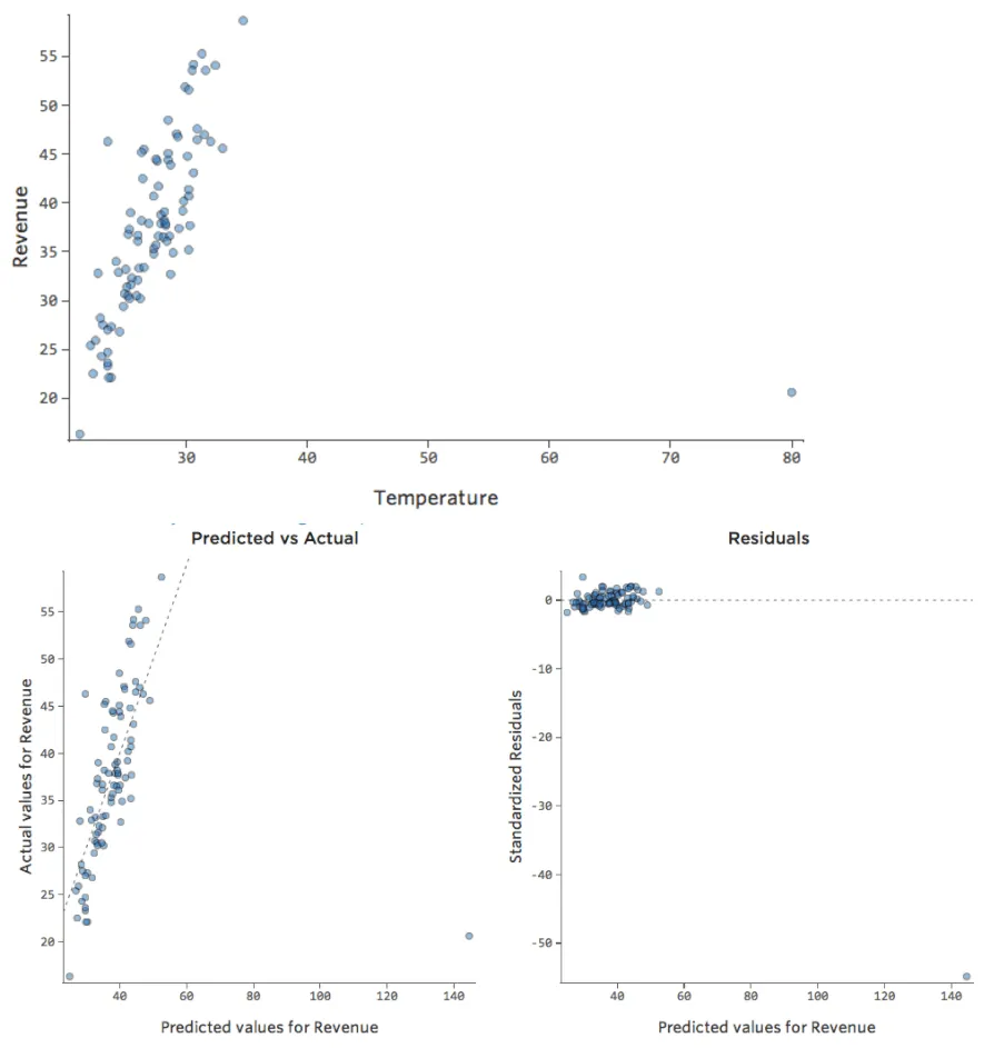
This regression has an outlying datapoint on an input variable, “Temperature” (outliers on an input variable are also known as “leverage points”).
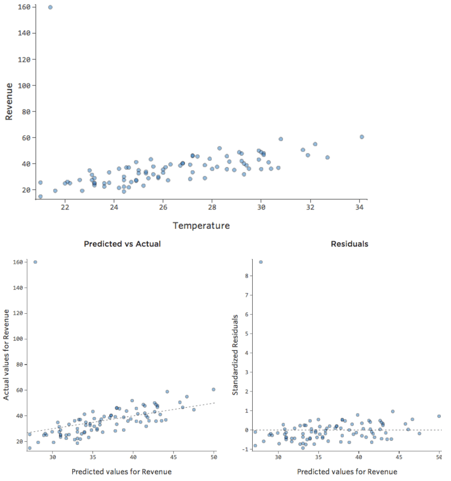
What if one of your datapoints had $160 in revenue instead of the normal $20 – $60? Your plots would look like this:
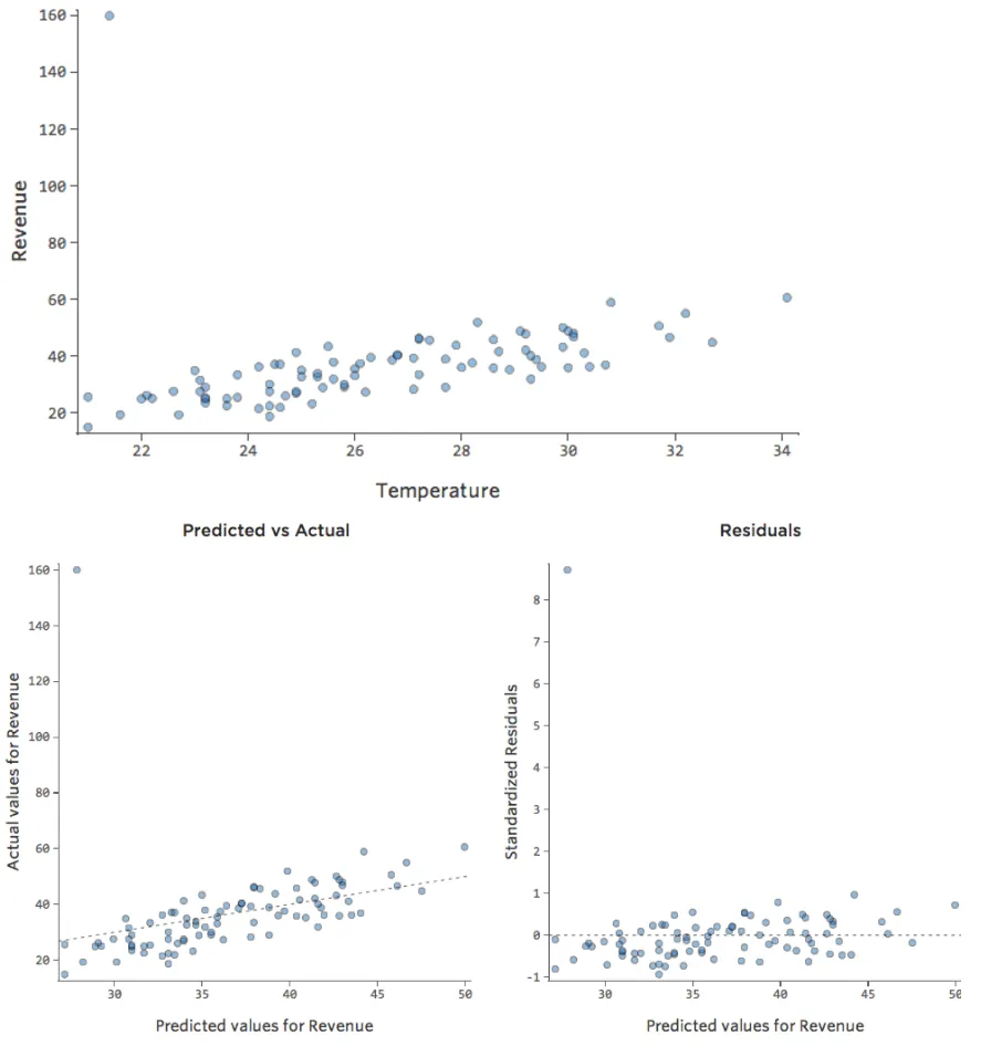
This regression has an outlying datapoint on an output variable, “Revenue.”
Implications
Stats iQ runs a type of regression that generally isn’t affected by output outliers (like the day with $160 revenue), but it is affected by input outliers (like a “Temperature” in the 80s). In the worst case, your model can pivot to try to get closer to that point at the expense of being close to all the others and end up being just entirely wrong, like this:
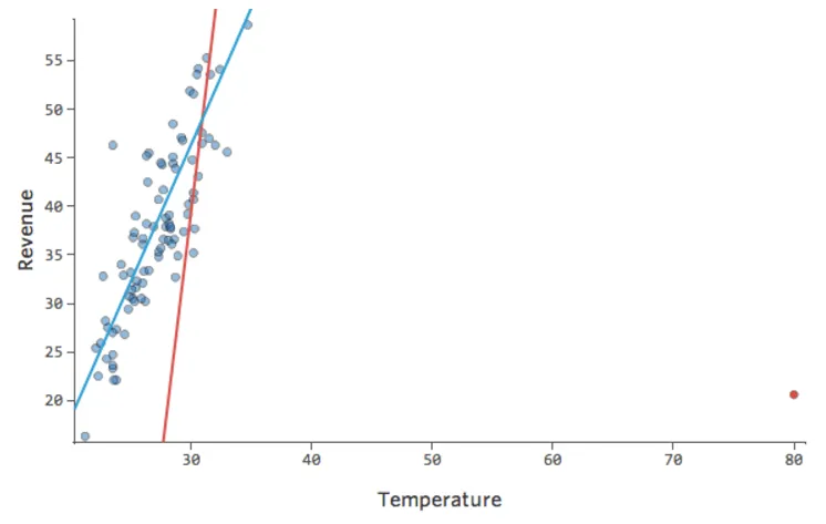
The blue line is probably what you’d want your model to look like, and the red line is the model you might see if you have that outlier out at “Temperature” 80.
How to Fix
- It’s possible that this is a measurement or data entry error, where the outlier is just wrong, in which case you should delete it.
- It’s possible that what appears to be just a couple outliers is in fact a power distribution. Consider transforming the variable if one of your variables has an asymmetric distribution (that is, it’s not remotely bell-shaped).
- If it is indeed a legitimate outlier, you should assess the impact of the outlier.
Large Y-axis Datapoints
Show details about this plot, and how to fix it.
Show details about this plot, and how to fix it.
Problem
Imagine that for whatever reason, your lemonade stand typically has low revenue, but every once and a while you get very high-revenue days, such that “Revenue” looked like this…
…instead of something more symmetrical and bell-shaped like this:
So “Temperature” vs. “Revenue” might look like this, with most of the data bunched at the bottom…
The black line represents the model equation, the model’s prediction of the relationship between “Temperature” and “Revenue.” Look above at each prediction made by the black line for a given “Temperature” (e.g., at “Temperature” 30, “Revenue” is predicted to be about 20). You can see that the majority of dots are below the line (that is, the prediction was too high), but a few dots are very far above the line (that is, the prediction was far too low).
Translating that same data to the diagnostic plots, most of the equation’s predictions are a bit too high, and then some would be way too low.
Implications
This almost always means your model can be made significantly more accurate. Most of the time you’ll find that the model was directionally correct but pretty inaccurate relative to an improved version. It’s not uncommon to fix an issue like this and consequently see the model’s r-squared jump from 0.2 to 0.5 (on a 0 to 1 scale).
How to Fix
- The solution to this is almost always to transform your data, typically your response variable.
- It’s also possible that your model lacks a variable.
Show details about this plot, and how to fix it.
Show details about this plot, and how to fix it.
Problem
These plots exhibit “heteroscedasticity,” meaning that the residuals get larger as the prediction moves from small to large (or from large to small).
Imagine that on cold days, the amount of revenue is very consistent, but on hotter days, sometimes revenue is very high and sometimes it’s very low.
You’d see plots like these:
Implications
This doesn’t inherently create a problem, but it’s often an indicator that your model can be improved.
The only exception here is that if your sample size is less than 250, and you can’t fix the issue using the below, your p-values may be a bit higher or lower than they should be, so possibly a variable that is right on the border of significance may end up erroneously on the wrong side of that border. Your regression coefficients (the number of units “Revenue” changes when “Temperature” goes up one) will still be accurate, though.
How to Fix
- The most frequently successful solution is to transform a variable.
- Often heteroscedasticity indicates that a variable is missing.
Show details about this plot, and how to fix it.
Show details about this plot, and how to fix it.
Problem
Imagine that it’s hard to sell lemonade on cold days, easy to sell it on warm days, and hard to sell it on very hot days (maybe because no one leaves their house on very hot days).
That plot would look like this:
The model, represented by the line, is terrible. The predictions would be way off, meaning your model doesn’t accurately represent the relationship between “Temperature” and “Revenue.”
Accordingly, residuals would look like this:
Implications
If your model is way off, as in the example above, your predictions will be pretty worthless (and you’ll notice a very low r-squared, like the 0.027 r-squared for the above).
Other times a slightly suboptimal fit will still give you a good general sense of the relationship, even if it’s not perfect, like the below:
That model looks pretty accurate. If you look closely (or if you look at the residuals), you can tell that there’s a bit of a pattern here – that the dots are on a curve that the line doesn’t quite match.
Does that matter? It’s up to you. If you’re getting a quick understanding of the relationship, your straight line is a pretty decent approximation. If you’re going to use this model for prediction and not explanation, the most accurate possible model would probably account for that curve.
How to Fix
- Sometimes patterns like this indicate that a variable needs to be transformed.
- If the pattern is actually as clear as these examples, you probably need to create a nonlinear model (it’s not as hard as that sounds).
- Or, as always, it’s possible that the issue is a missing variable.
Show details about this plot, and how to fix it.
Show details about this plot, and how to fix it.
Problem
What if one of your datapoints had a “Temperature” of 80 instead of the normal 20s and 30s? Your plots would look like this:
This regression has an outlying datapoint on an input variable, “Temperature” (outliers on an input variable are also known as “leverage points”).
What if one of your datapoints had $160 in revenue instead of the normal $20 – $60? Your plots would look like this:
This regression has an outlying datapoint on an output variable, “Revenue.”
Implications
Stats iQ runs a type of regression that generally isn’t affected by output outliers (like the day with $160 revenue), but it is affected by input outliers (like a “Temperature” in the 80s). In the worst case, your model can pivot to try to get closer to that point at the expense of being close to all the others and end up being just entirely wrong, like this:
The blue line is probably what you’d want your model to look like, and the red line is the model you might see if you have that outlier out at “Temperature” 80.
How to Fix
- It’s possible that this is a measurement or data entry error, where the outlier is just wrong, in which case you should delete it.
- It’s possible that what appears to be just a couple outliers is in fact a power distribution. Consider transforming the variable if one of your variables has an asymmetric distribution (that is, it’s not remotely bell-shaped).
- If it is indeed a legitimate outlier, you should assess the impact of the outlier.
Show details about this plot, and how to fix it.
Show details about this plot, and how to fix it.
Problem
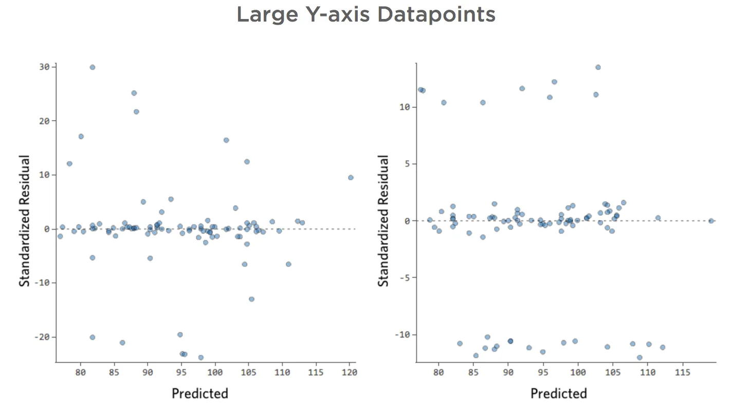
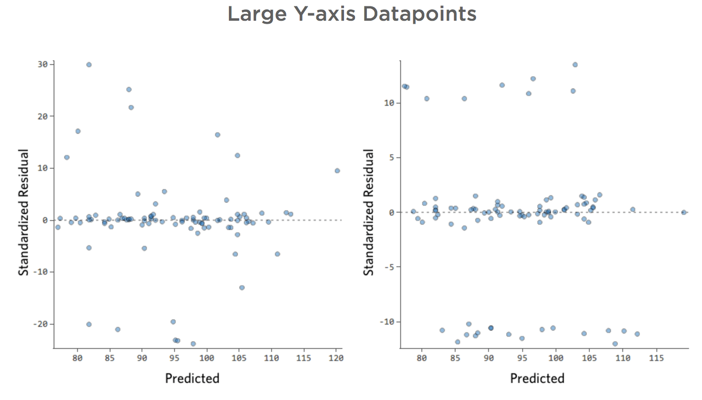
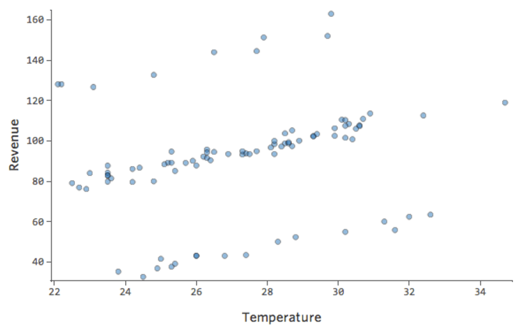
Imagine that there are two competing lemonade stands nearby. Most of the time only one is operational, in which case your revenue is consistently good. Sometimes neither is active and revenue soars; at other times, both are active and revenue plummets.
“Revenue” vs. “Temperature” might look like this…
…with that top row being days when no other stand shows up and the bottom row being days when both other stands are in business.
That’d result in these residual plots:

That is, there’s quite a few datapoints on both sides of 0 that have residuals of 10 or higher, which is to say that the model was way off.
Now if you’d collected data every day for a variable called “Number of active lemonade stands,” you could add that variable to your model and this problem would be fixed. But often you don’t have the data you need (or even a guess as to what kind of variable you need).
Implications
Your model isn’t worthless, but it’s definitely not as good as if you had all the variables you needed. You could still use it and you might say something like, “This model is pretty accurate most of the time, but then every once and a while it’s way off.” Is that useful? Probably, but that’s your decision and it depends on what decisions you’re trying to make based on your model.
How to Fix
- Even though this approach wouldn’t work in the specific example above, it’s almost always worth looking around to see if there’s an opportunity to usefully transform a variable.
- If that doesn’t work though, you probably need to deal with your missing variable problem.
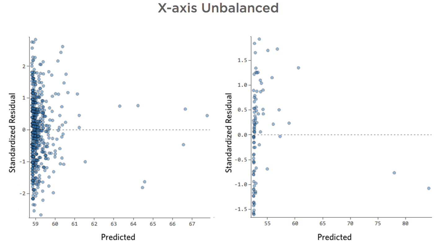
X-axis Unbalanced
Show details about this plot, and how to fix it.
Show details about this plot, and how to fix it.
Problem
Imagine that for whatever reason, your lemonade stand typically has low revenue, but every once and a while you get very high-revenue days, such that “Revenue” looked like this…
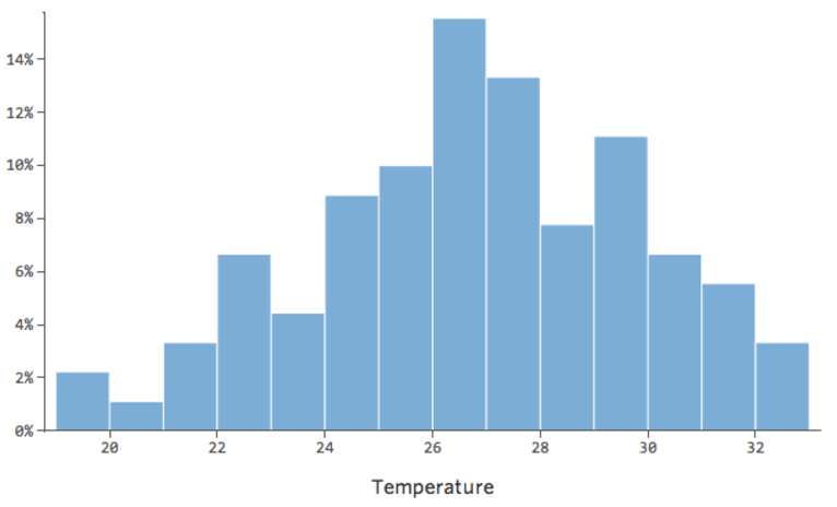
…instead of something more symmetrical and bell-shaped like this:
So “Temperature” vs. “Revenue” might look like this, with most of the data bunched at the bottom…
The black line represents the model equation, the model’s prediction of the relationship between “Temperature” and “Revenue.” Look above at each prediction made by the black line for a given “Temperature” (e.g., at “Temperature” 30, “Revenue” is predicted to be about 20). You can see that the majority of dots are below the line (that is, the prediction was too high), but a few dots are very far above the line (that is, the prediction was far too low).
Translating that same data to the diagnostic plots, most of the equation’s predictions are a bit too high, and then some would be way too low.
Implications
This almost always means your model can be made significantly more accurate. Most of the time you’ll find that the model was directionally correct but pretty inaccurate relative to an improved version. It’s not uncommon to fix an issue like this and consequently see the model’s r-squared jump from 0.2 to 0.5 (on a 0 to 1 scale).
How to Fix
- The solution to this is almost always to transform your data, typically your response variable.
- It’s also possible that your model lacks a variable.
Show details about this plot, and how to fix it.
Show details about this plot, and how to fix it.
Problem
These plots exhibit “heteroscedasticity,” meaning that the residuals get larger as the prediction moves from small to large (or from large to small).
Imagine that on cold days, the amount of revenue is very consistent, but on hotter days, sometimes revenue is very high and sometimes it’s very low.
You’d see plots like these:
Implications
This doesn’t inherently create a problem, but it’s often an indicator that your model can be improved.
The only exception here is that if your sample size is less than 250, and you can’t fix the issue using the below, your p-values may be a bit higher or lower than they should be, so possibly a variable that is right on the border of significance may end up erroneously on the wrong side of that border. Your regression coefficients (the number of units “Revenue” changes when “Temperature” goes up one) will still be accurate, though.
How to Fix
- The most frequently successful solution is to transform a variable.
- Often heteroscedasticity indicates that a variable is missing.
Show details about this plot, and how to fix it.
Show details about this plot, and how to fix it.
Problem
Imagine that it’s hard to sell lemonade on cold days, easy to sell it on warm days, and hard to sell it on very hot days (maybe because no one leaves their house on very hot days).
That plot would look like this:
The model, represented by the line, is terrible. The predictions would be way off, meaning your model doesn’t accurately represent the relationship between “Temperature” and “Revenue.”
Accordingly, residuals would look like this:
Implications
If your model is way off, as in the example above, your predictions will be pretty worthless (and you’ll notice a very low r-squared, like the 0.027 r-squared for the above).
Other times a slightly suboptimal fit will still give you a good general sense of the relationship, even if it’s not perfect, like the below:
That model looks pretty accurate. If you look closely (or if you look at the residuals), you can tell that there’s a bit of a pattern here – that the dots are on a curve that the line doesn’t quite match.
Does that matter? It’s up to you. If you’re getting a quick understanding of the relationship, your straight line is a pretty decent approximation. If you’re going to use this model for prediction and not explanation, the most accurate possible model would probably account for that curve.
How to Fix
- Sometimes patterns like this indicate that a variable needs to be transformed.
- If the pattern is actually as clear as these examples, you probably need to create a nonlinear model (it’s not as hard as that sounds).
- Or, as always, it’s possible that the issue is a missing variable.
Show details about this plot, and how to fix it.
Show details about this plot, and how to fix it.
Problem
What if one of your datapoints had a “Temperature” of 80 instead of the normal 20s and 30s? Your plots would look like this:
This regression has an outlying datapoint on an input variable, “Temperature” (outliers on an input variable are also known as “leverage points”).
What if one of your datapoints had $160 in revenue instead of the normal $20 – $60? Your plots would look like this:
This regression has an outlying datapoint on an output variable, “Revenue.”
Implications
Stats iQ runs a type of regression that generally isn’t affected by output outliers (like the day with $160 revenue), but it is affected by input outliers (like a “Temperature” in the 80s). In the worst case, your model can pivot to try to get closer to that point at the expense of being close to all the others and end up being just entirely wrong, like this:
The blue line is probably what you’d want your model to look like, and the red line is the model you might see if you have that outlier out at “Temperature” 80.
How to Fix
- It’s possible that this is a measurement or data entry error, where the outlier is just wrong, in which case you should delete it.
- It’s possible that what appears to be just a couple outliers is in fact a power distribution. Consider transforming the variable if one of your variables has an asymmetric distribution (that is, it’s not remotely bell-shaped).
- If it is indeed a legitimate outlier, you should assess the impact of the outlier.
Show details about this plot, and how to fix it.
Show details about this plot, and how to fix it.
Problem
Imagine that there are two competing lemonade stands nearby. Most of the time only one is operational, in which case your revenue is consistently good. Sometimes neither is active and revenue soars; at other times, both are active and revenue plummets.
“Revenue” vs. “Temperature” might look like this…
…with that top row being days when no other stand shows up and the bottom row being days when both other stands are in business.
That’d result in these residual plots:
That is, there’s quite a few datapoints on both sides of 0 that have residuals of 10 or higher, which is to say that the model was way off.
Now if you’d collected data every day for a variable called “Number of active lemonade stands,” you could add that variable to your model and this problem would be fixed. But often you don’t have the data you need (or even a guess as to what kind of variable you need).
Implications
Your model isn’t worthless, but it’s definitely not as good as if you had all the variables you needed. You could still use it and you might say something like, “This model is pretty accurate most of the time, but then every once and a while it’s way off.” Is that useful? Probably, but that’s your decision and it depends on what decisions you’re trying to make based on your model.
How to Fix
- Even though this approach wouldn’t work in the specific example above, it’s almost always worth looking around to see if there’s an opportunity to usefully transform a variable.
- If that doesn’t work though, you probably need to deal with your missing variable problem.
Show details about this plot, and how to fix it.
Show details about this plot, and how to fix it.
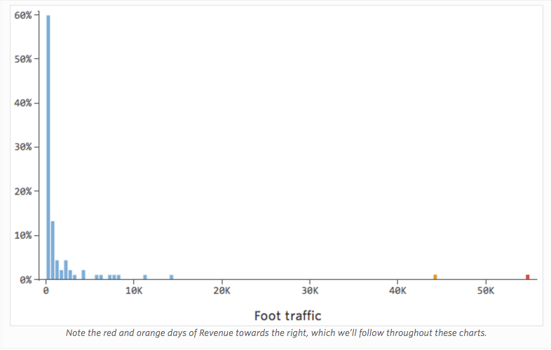
Problem
Imagine that “Revenue” is driven by nearby “Foot traffic,” in addition to or instead of just “Temperature.” Imagine that, for whatever reason, your lemonade stand typically has low revenue, but every once and a while you get extremely high-revenue days such that your revenue looked like this…


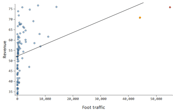
So “Foot traffic” vs. “Revenue” might look like this, with most of the data bunched on the left side:
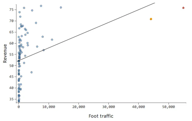
The black line represents the model equation, the model’s prediction of the relationship between “Foot traffic” and “Revenue.” You can see that the model can’t really tell the difference between “Foot traffic” of 0 and of, say, 100 or 1,000; for each of those values it would predict revenue near $53.
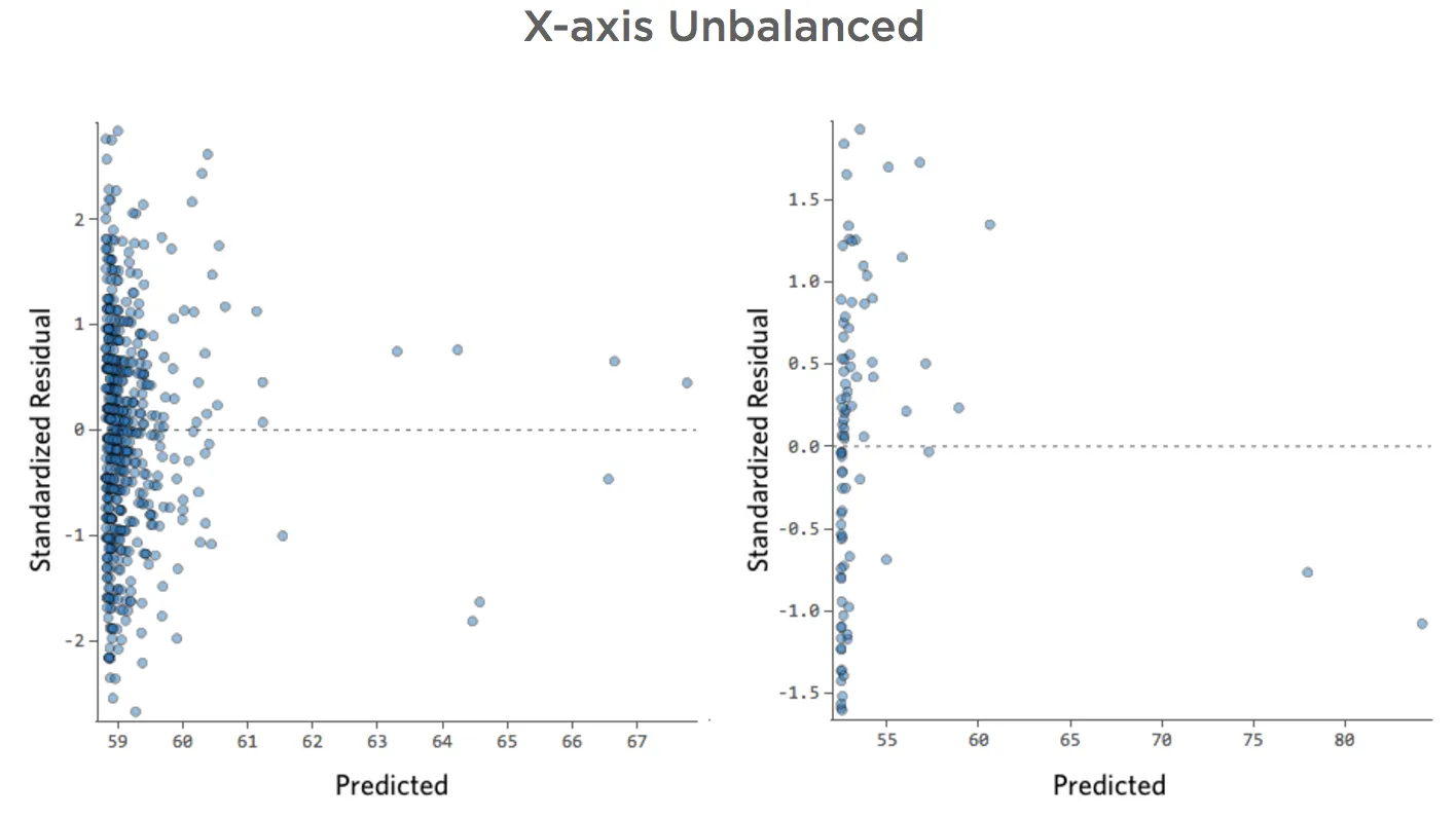
Translating that same data to the diagnostic plots:
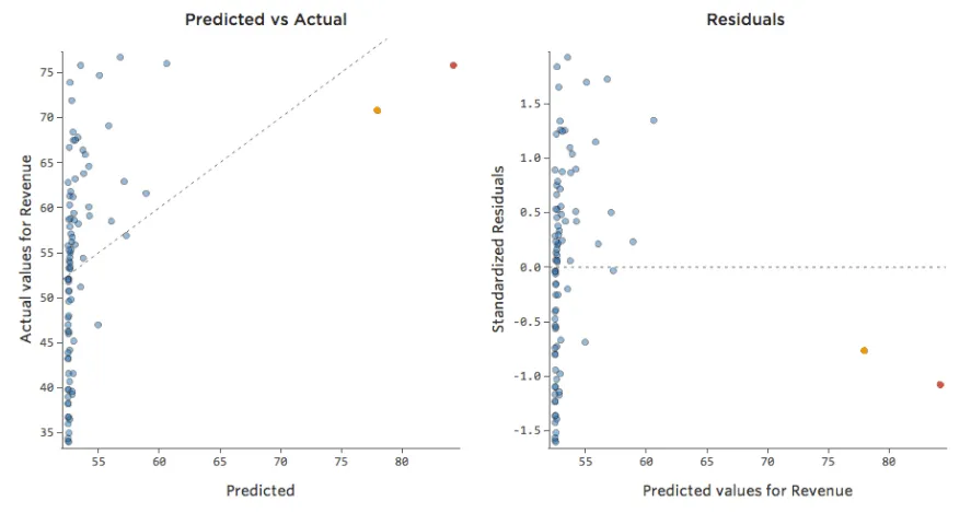
Implications
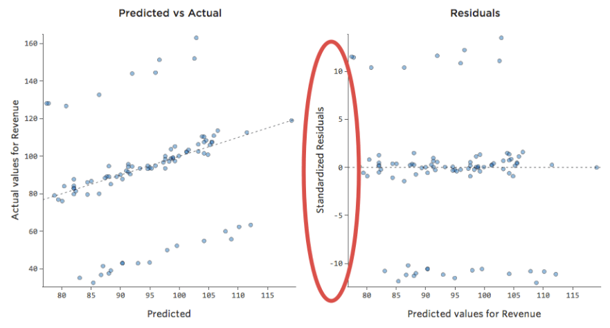
Sometimes there’s actually nothing wrong with your model. In the above example, it’s quite clear that this isn’t a good model, but sometimes the residual plot is unbalanced and the model is quite good.
The only ways to tell are to a) experiment with transforming your data and see if you can improve it and b) look at the predicted vs. actual plot and see if your prediction is wildly off for a lot of datapoints, as in the above example (but unlike the below example).
While there’s no explicit rule that says your residual can’t be unbalanced and still be accurate (indeed this model is quite accurate), it’s more often the case that an x-axis unbalanced residual means your model can be made significantly more accurate. Most of the time you’ll find that the model was directionally correct but pretty inaccurate relative to an improved version. It’s not uncommon to fix an issue like this and consequently see the model’s r-squared jump from 0.2 to 0.5 (on a 0 to 1 scale).
How to Fix
- The solution to this is almost always to transform your data, typically an explanatory variable. (Note that the example shown below will reference transforming your response variable, but the same process will be helpful here.)
- It’s also possible that your model lacks a variable.
Improving Your Model: Assessing the Impact of an Outlier
Let’s assume that you have an outlying datapoint that is legitimate, not a measurement or data error. To decide how to move forward, you should assess the impact of the datapoint on the regression.
The easiest way to do this is to note the coefficients of your current model, then filter out that datapoint from the regression. If the model doesn’t change much, then you don’t have much to worry about.
If that changes the model significantly, examine the model (particularly actual vs. predicted), and decide which one feels better to you. It’s okay to ultimately discard the outlier as long as you can theoretically defend that, saying, “In this case we’re not interested in outliers, they’re just not of interest,” or “That was the day Uncle Jerry came buy and tipped me $100; that’s not predictable, and it’s not worth including in the model.”
Improving Your Model: Transforming Variables
Overview
The most common way to improve a model is to transform one or more variables, usually using a “log” transformation.
Transforming a variable changes the shape of its distribution. Typically the best place to start is a variable that has an asymmetrical distribution, as opposed to a more symmetrical or bell-shaped distribution. So find a variable like this to transform:
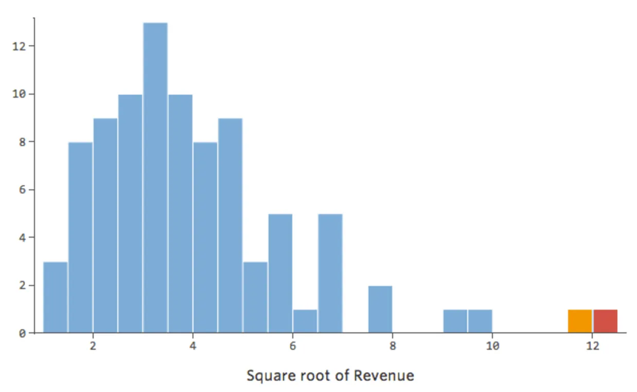
In general, regression models work better with more symmetrical, bell-shaped curves. Try different kinds of transformations until you hit upon the one closest to that shape. It’s often not possible to get close to that, but that’s the goal. So let’s say you take the square root of “Revenue” as an attempt to get to a more symmetrical shape, and your distribution looks like this:
That’s good, but it’s still a bit asymmetrical. Let’s try taking the log of “Revenue” instead, which yields this shape:
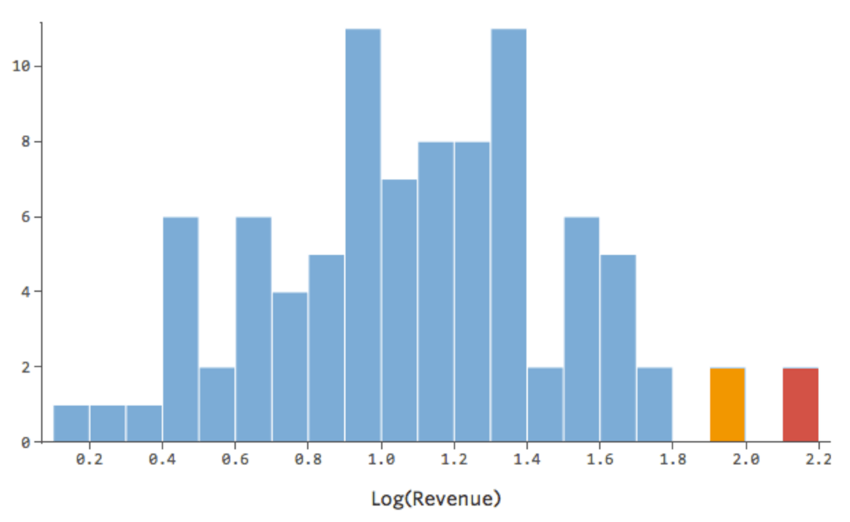
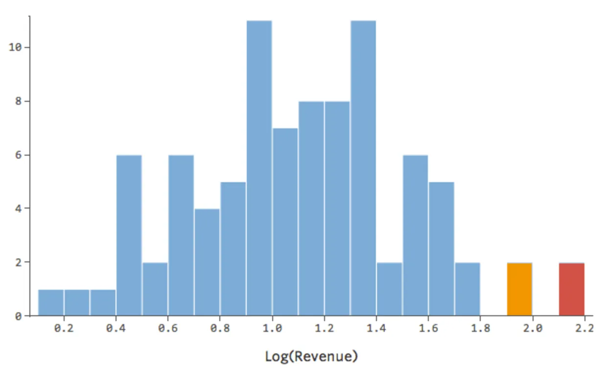
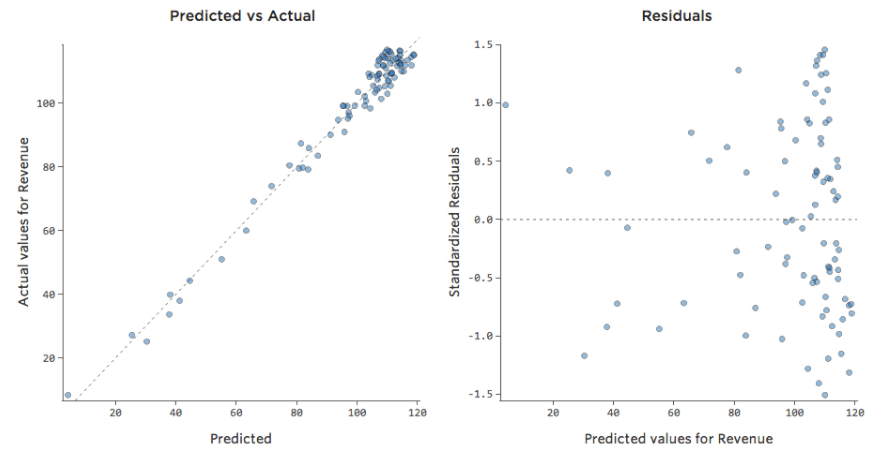
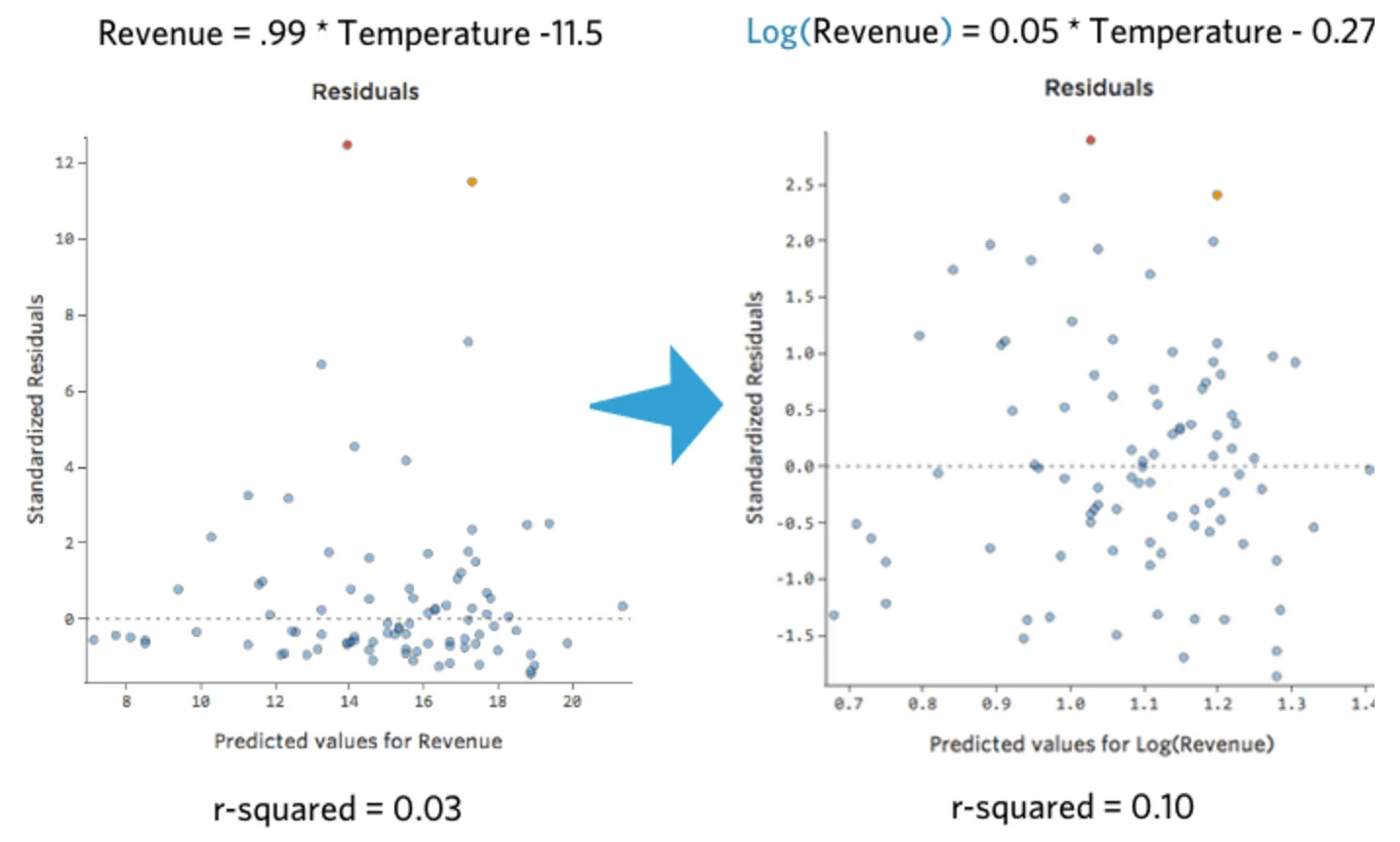
That’s nice and symmetrical. You’re probably going to get a better regression model with log(“Revenue”) instead of “Revenue.” Indeed, here’s how your equation, your residuals, and your r-squared might change:
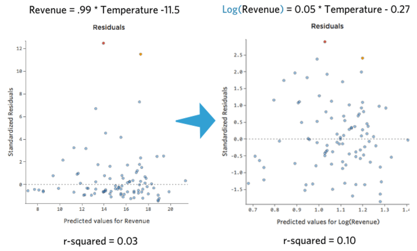
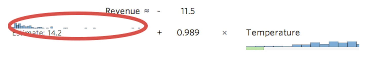
Stats iQ shows a small version of the variable’s distribution inline with the regression equation:
Select the transformation fx button to the left of the variable…
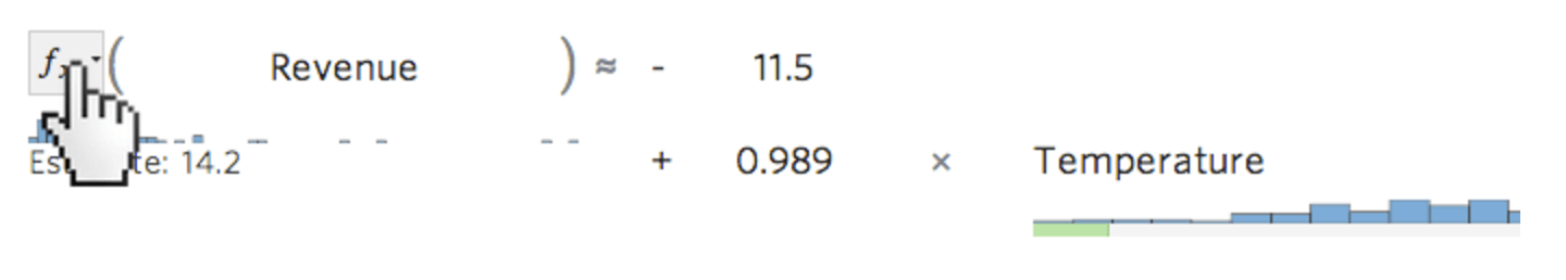

…then select a transformation, most often log(x)...
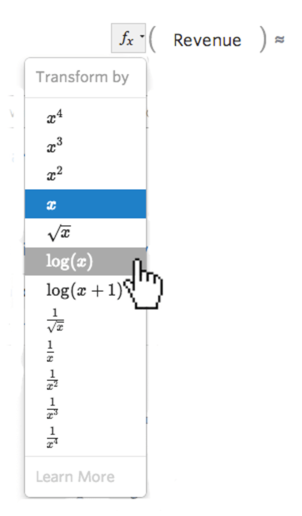

…then examine the histogram to see if it’s more centered, as this one is after transformation:
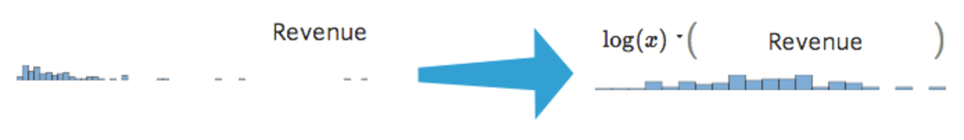

After transforming a variable, note how its distribution, the r-squared of the regression, and the patterns of the residual plot change. If those improve (particularly the r-squared and the residuals), it’s probably best to keep the transformation.
If a transformation is necessary, you should start by taking a “log” transformation because the results of your model will still be easy to understand. Note that you’ll run into issues if the data you’re trying to transform includes zeros or negative values, though. To learn why taking a log is so useful, or if you have non-positive numbers you want to transform, or if you just want to get a better understanding of what’s happening when you transform data, read on through the details below.
Details
If you take the log10() of a number, you’re saying “10 to what power gives me that number.” For example, here’s a simple table of four datapoints, including both “Revenue” and Log(“Revenue”):
| Temperature | Revenue | Log(Revenue) |
|---|---|---|
| 20 | 100 | 2 |
| 30 | 1,000 | 3 |
| 40 | 10,000 | 4 |
| 45 | 31,623 | 4.5 |
Note that if we plot “Temperature” vs. “Revenue,” and “Temperature” vs. Log(“Revenue”), the latter model fits much better.
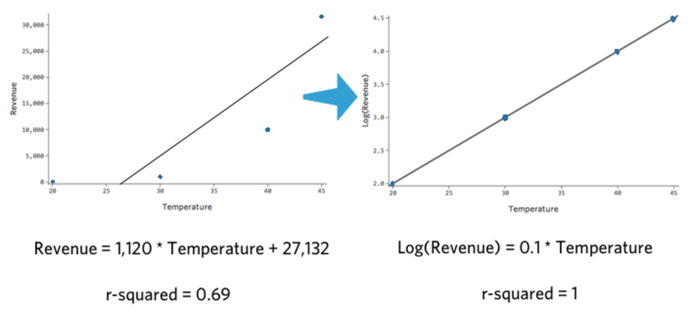
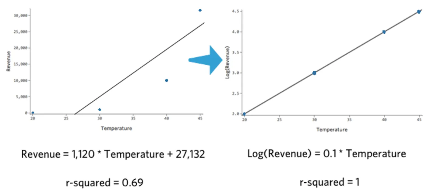
The interesting thing about this transformation is that your regression is no longer linear. When “Temperature” went from 20 to 30, “Revenue” went from 10 to 100, a 90-unit gap. Then when “Temperature” went from 30 to 40, “Revenue” went from 100 to 1000, a much larger gap.
If you’ve taken a log of your response variable, it’s no longer the case that a one-unit increase in “Temperature” means a X–unit increase in “Revenue.” Now it’s a X–percent increase in “Revenue.” In this case, a ten-unit increase in “Temperature” is associated with a 1000% increase in Y – that is, a one-unit increase in “Temperature” is associated with a 26% increase in “Revenue.”
Also note that you can’t take the log of 0 or of a negative number (there is no X where 10X = 0 or 10X= -5), so if you do a log transformation, you’ll lose those datapoints from the regression. There’s 4 common ways of handling the situation:
Improving Your Model: Missing Variables
Probably the most common reason that a model fails to fit is that not all the right variables are included. This particular issue has a lot of possible solutions.
Adding a New Variable
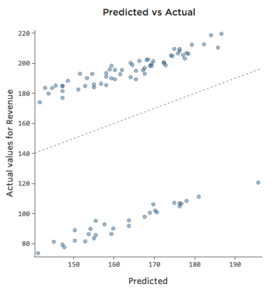
Sometimes the fix is as easy as adding another variable to the model. For example, if lemonade stand “Revenue” traffic was much larger on weekends than weekdays, your predicted vs. actual plot might look like the below (r-squared of 0.053) since the model is just taking the average of weekend days and weekdays:
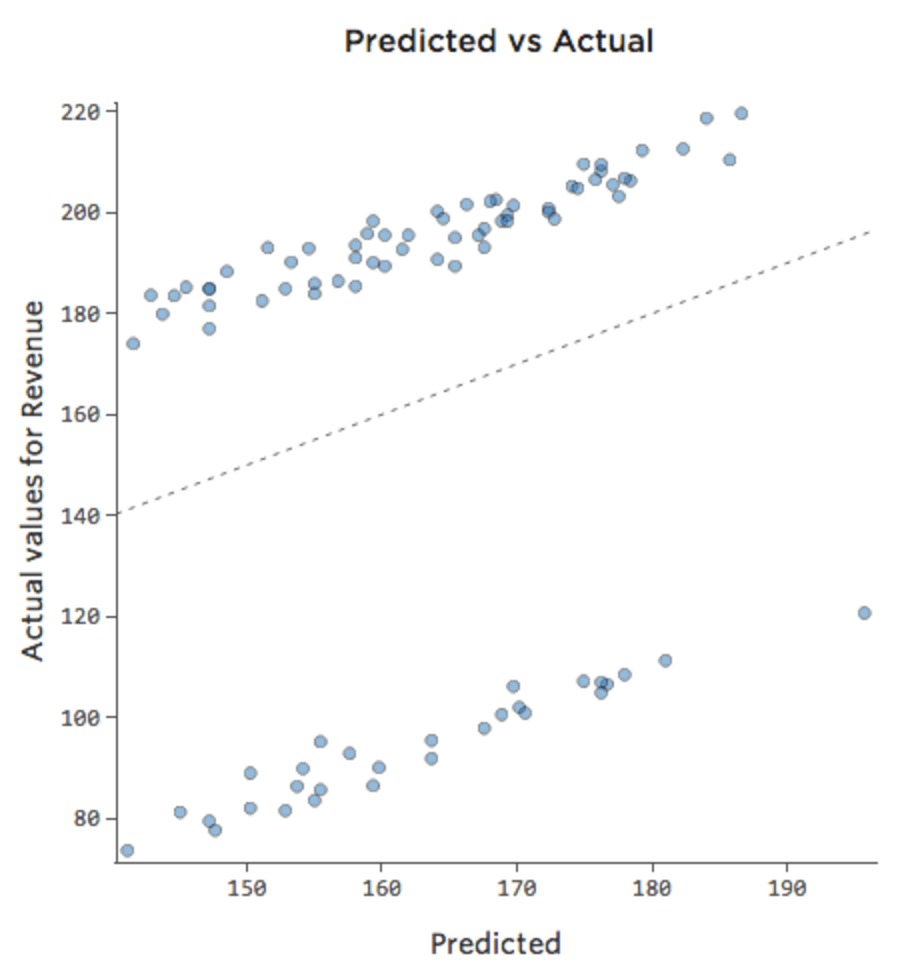
If the model includes a variable called “Weekend,” then the predicted vs. actual plot might look like this (r-squared of 0.974):
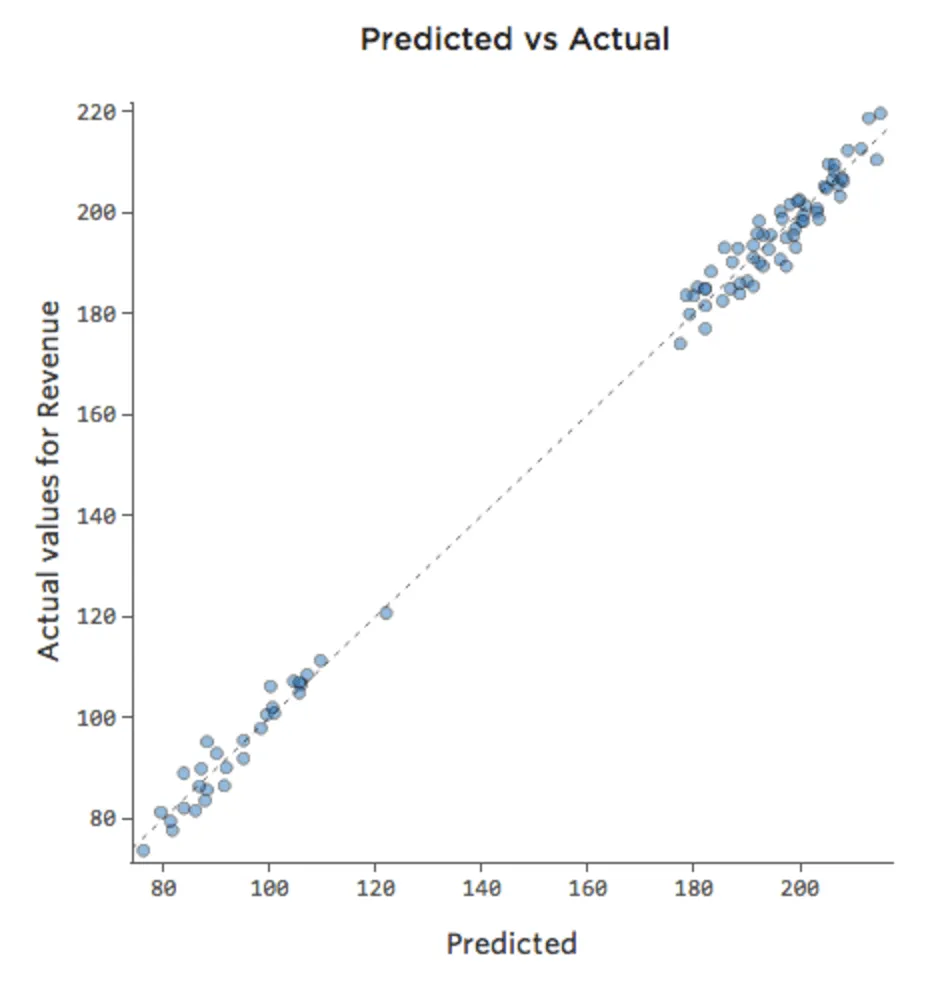
The model makes far more accurate predictions because it’s able to take into account whether a day of the week is a weekday or not.
Note that sometimes you’ll need to create variables in Stats iQ to improve your model in this fashion. For example, you might have had a “Date” variable (with values like “10/26/2014”) and you might need to create a new variable called “Day of Week” (i.e., Sunday) or Weekend (i.e., Weekend).
Unavailable Omitted Variable
It’s rarely that easy, though. Quite frequently the relevant variable isn’t available because you don’t know what it is or it was difficult to collect. Maybe it wasn’t a weekend vs. weekday issue, but instead something like “Number of Competitors in the Area” that you failed to collect at the time.
If the variable you need is unavailable, or you don’t even know what it would be, then your model can’t really be improved and you have to assess it and decide how happy you are with it (whether it’s useful or not, even though it’s flawed).
Interactions Between Variables
Perhaps on weekends the lemonade stand is always selling at 100% of capacity, so regardless of the “Temperature,” “Revenue” is high. But on weekdays, the lemonade stand is much less busy, so “Temperature” is an important driver of “Revenue.” If you ran a regression that included “Weekend” and “Temperature,” you might see a predicted vs. actual plot like this, where the row along the top are the weekend days.
We would say that there’s an interaction between “Weekend” and “Temperature”; the effect of one of them on “Revenue” is different based on the value of the other. If we create an interaction variable, we get a much better model, where predicted vs. actual looks like this:
Improving Your Model: Fixing Nonlinearity
Let’s say you have a relationship that looks like this:
You might notice that the shape is that of a parabola, which you might recall is typically associated with formulas that look like this:
y = x2 + x + 1
By default, regression uses a linear model that looks like this:
y = x + 1
In fact, the line in the plot above has this formula:
y = 1.7x + 51
But it’s a terrible fit. So if we add an x2 term, our model has a better chance of fitting the curve. In fact, it creates this:

The formula for that curve is:
y = -2x2 +111x – 1408
That means our diagnostic plots change from this…
…to this:
Note that these are healthy diagnostic plots, even though the data appears to be unbalanced to the right side of it.
The above approach can be extended to other kinds of shapes, particularly an S-shaped curve, by adding an x3 term. That’s relatively uncommon, though.
A few cautions:
- Generally speaking, if you have an x2 term because of a nonlinear pattern in your data, you want to have a plain-old-x-not-x2 term. You may find that your model is perfectly good without it, but you should definitely try both to start.
- The regression equation may be difficult to understand. For the linear equation at the beginning of this section, for each additional unit of “Temperature,” “Revenue” went up 1.7 units. When you have both x2 and x in the equation, it’s not easy to say “When Temperature goes up one degree, here’s what happens.” Sometimes for that reason it’s easier to just use a linear equation, assuming that equation fits well enough.
FAQs
How do I create a new Stats iQ variable?
How do I create a new Stats iQ variable?
What are the options for analyzing my data in Stats iQ?
What are the options for analyzing my data in Stats iQ?
- Describe: Selecting a variable from the list and then clicking Describe will give you a visualization of the data contained in that variable. Use this when you would like to see how the data for a certain variable is distributed.
- Relate: Selecting two variables and then clicking Relate will run a statistical analysis of the relation between the two variables. Use this when you would like to know how strongly two variables are correlated.
- Pivot Table: Selecting two or more variables and clicking Pivot Table will create a table that displays the values of the variables as rows and columns. The cells can be set to display a variety of different information including column and row percentage, Sum, and Variance. Use this when you would like to compare the overlap between specific values of a set of variables.
- Regression: Selecting two variables and clicking Regression will give the mathematical relationship between the variables. Use this when you would like to predict values for one variable based off of the values of another.
- Cluster: Selecting two to ten demographic variables and clicking Cluster will display groupings of traits most likely to occur together, thus revealing the population segments captured in your data.
I don't know what this statistical term means. Can you tell me?
I don't know what this statistical term means. Can you tell me?
- Statistical tests: ANOVA, T-test, and Chi-squared are all statistical test that Stats iQ performs to test whether or not the relationship between two variables is significant. These tests are used to generate a P-Value.
- P-Value: This value represents the probability that the observed results would be seen if no correlation between the variables exists. A lower P-Value means more correlated data.
- Effect Size: The effect size is a measure of how large the correlation between two variables is. This is measured in different ways depending on the type of the statistical test performed. Examples are Cohen’s d, Pearson’s r, and Cramer’s v. The larger the effect size value, the more correlated the variables are.
How do I filter the data that appears in Stats iQ?
How do I filter the data that appears in Stats iQ?
How do I get my new responses to show up in Stats iQ?
How do I get my new responses to show up in Stats iQ?
How are analysis cards ordered in my Stats iQ Workspace?
How are analysis cards ordered in my Stats iQ Workspace?
What’s Stats iQ? / Where’s Statwing?
What’s Stats iQ? / Where’s Statwing?
What do I do if my data isn't loading properly?
What do I do if my data isn't loading properly?
That's great! Thank you for your feedback!
Thank you for your feedback!